My system/room was measured for the first time at the end of 2013. At that time I still had a purely analogue setup with the Stacked Quads and the RiPol. I split the frequency with the AFW1 at 125Hz. Of course I had a few ideas at that time about what could be improved, but overall I was satisfied.
This measurement changed everything!
It mercilessly showed me what was wrong and what compromises I had been listening to all those years.
This led to the development of the active absorber in the following years and the changeover to digital signal processing in 2021. Since then, I have been learning more and more, with some astonishing improvements in the playback quality in my listening room.
In addition to the possibility of implementing room acoustics measures, I was also inspired by the article
Dr. Ulrich Brüggemann – Thoughts About Crossovers
to follow this path. When you realise how inadequate analogue crossovers are and how much better digital FIR filters can do the job, then you simply have to draw the consequences. You can find the article in the Infocenter on the AudioVero homepage.
Digital signal reproduction also offers the option of time alignment in a multi-way system. A music signal that is split between the speakers and does not reach the ear at the same time is not reproduced correctly per se.
In the following I describe the way I currently use to measure my setup in order to determine the correction files. I hope that I can give other users of Acourate and the AcourateConvolver suggestions and a guide on how to approach optimisation.
A very good introduction to Acourate can be found in the manual “Quick introduction to Acourate”, which can be found in the info centre on the AudioVero homepage as a pdf file.
The following book is also a good choice:
Mitch Barnett – Accurate Sound Reproduction Using DSP
However, Mitch uses JRiver and there is no information about the AcourateConvolver. Nevertheless, a lot of technical and acoustic background is explained. You can get it as a book or as a Kindle eBook. Even though I don’t use JRiver myself, I found the book extremely informative.
In the following, you will also repeatedly come across recommendations, settings or measurements from Mitch.
The hardware and software components used determine the procedure for the Acourate optimisation of your own system, at least in some areas. Therefore, individual differences may occur.
The system is quite complex and therefore prone to errors. It requires knowledge of digital signal processing. But you also need to know how to administer computers and networks and how to set up an operating system. If things get stuck in one place and you don’t have the necessary knowledge, it can very quickly put an end to relaxed music listening via an optimised audio playback system. However, if everything works as intended, you get a reproduction with a quality that you never thought possible.
The effort is definitely worth it!
It’s best to find someone to mentor you. This makes it much easier to get started.
Description of the Components
June 11, 2024
One of the most important software components that I use alongside the actual Acourate is the AcourateConvolver. In some places, this has a direct effect on how the calculated parameters and correction files are processed. But it also determines the topology of the hardware.
Hardware Used
At the centre of my audio signal processing sits a Lynx Aurora(n) studio converter. This converter has a modular design, so this statement needs to be specified in more detail: It is a “PRE 2016 DANTE”. This means that the converter is equipped with 16 analogue inputs and outputs and 4 microphone inputs on the analogue side. For digital signal transfer, it is equipped with a card for connection to a Dante network.
The AcourateConvolver runs on a PC with an Intel Core i7-13700K with 16GB RAM. I use a Windows Server 2022 Standard for 24 cores as the operating system. My experience has shown me that it is beneficial for the audio performance if the computer has as little to do as possible, hence the powerful CPU and the server operating system. The computer runs without a mouse, keyboard and monitor. It is administered remotely by me. The computer is equipped with 2 Ethernet interfaces. The first is connected to my private network and the second is used to connect to the Dante network. As the computer is located in an adjoining room, it can be actively cooled. This means that I am not limited to 65W types that can still be passively cooled when selecting the CPU.
The centre of the Dante network is a Cisco SG250-08 managed switch. I use the Dante network exclusively for the audio data transmission. The settings of the switch are optimised for the transfer of audio data in the Dante network. I use CAT6 cables.
In an active multi-way system described here, the volume should/must be controlled after the convolution (AcourateConvolver). For this reason, a corresponding multi-channel preamplifier is required. I use my VV7 preamplifier at this point. The power amplifiers are connected to the outputs of the preamplifier. These drive the individual loudspeaker components of my RQM system. There are currently seven channels.
There is a second PC in my setup. It is passively cooled and is located directly in the listening room. The processor used is an Intel Core i5-10600 with 16GB RAM. Windows 11 Pro is running on this computer. The computer is equipped with a mouse, keyboard and monitor. This computer also has 2 Ethernet interfaces (internal network & Dante). I use this computer for the Acourate measurements and the administration of the Convolver PC, the Lynx converter and the Dante network.
The influence of the measuring equipment should not be underestimated! You can’t correct what you can’t capture with a cheap measuring microphone, for example. This is like comparing a cheap audio system with a high-resolution high-end system. A correction file for the microphone won’t help either, it only corrects the frequency response and doesn’t improve the resolution. I initially used such a microphone (<€100) and now use an Earthworks M50, the differences were more than clear to hear. The same applies to the rest of the measurement channel. And of course there is also a correction file for an Earthworks microphone. Nevertheless, you can of course carry out the first tests with inexpensive measurement equipment.
Software Used
As I mentioned in the description above, I also use the AcourateConvolver in addition to Acourate.
To integrate the two PCs into the Dante network, the Dante Virtual Soundcard (DVS) runs on the computers. It establishes the connection between the audio software and the Ethernet interface / Dante network via an ASIO interface. My Roon server is also integrated into the Dante network in this way.
The Dante Controller software is also installed on the measurement PC. This is used for the complete administration of the Dante network and the associated components.
The Lynx NControl software can also be found on this computer. This can be used to configure the converter. The connection is made via the Dante network, so no further hardware is required.
Optimization of the RQM System
March 17, 2026
Below, I describe the procedure for calibrating my RQM system. However, this procedure is not limited to my system, and most of it can be followed as described. Text between two dashes consists either of notes on specific settings and procedures for my system or technical explanations that provide further insight but do not necessarily need to be read.
At the time of writing this page I was using Acourate version 2.1.6 and AcourateConvolver version 2.0.7. I updated to Acourate version 3.1.0 and to AcourateConvover version 2.2.2 in August 2024.
I operate the Dante network at 96kHz / 24Bit. This setting turned out to be the “sweet spot” for me with my system. At higher frequencies I find the audio playback somewhat “strained”. I also carry out all measurements at this sample rate.
The Lynx converter is the clock master in my Dante network.
I create a separate directory with the current date in the name for each measurement. This gives me a chronological history. I also make notes on the measurements and the results. I use Joplin for this. So I can see what I have tried out on the system at any time.
At this point I have to anticipate a little. I operate my system with a filter length of 262144 taps. This is the largest possible number that can be set in Acourate. The recommendation for 96kHz is 131072 taps, but it simply sounds better to me this way.
Since the resonances in a room can sometimes be extremely narrow, FIR filters must have sufficient frequency resolution. The underlying mathematical principle is relatively simple.
fS is the sample rate and N is the filter length. With a clock frequency of 96kHz and a filter length of 262144 taps, this results in:
With the recommended filter length of 131072 taps at 96kHz, the frequency resolution is halved to 0.732Hz. I can hear the difference very clearly, especially in the lower frequency range.
That is also why solutions using low-cost DSPs do not work well. Their technical capabilities are generally far too limited (e.g., 48kHz with 8192 taps).
Incidentally, the term “tap” is derived from “to tap”, since in FIR filters, intermediate values are tapped from the delay line.
Before the system can be optimized, the signal routing in the Dante network must first be defined. Without correct routing, the system will not be able to produce any sound. Of course, this also applies to all other digital solutions. However, a description is not part of this document.
I also assume that Acourate and AcourateConvolver are installed and licensed. This means that everything is ready to use from the software side.
The following description is chronological and should be carried out as such.
Creation of the Calibration File for the Microphone Used
April 9, 2024
Every reputable manufacturer of a measurement microphone provides individual calibration data. This data is used to generate a correction file for the measurement with Acourate. It is integrated into the measurements in order to correct the microphone’s inaccuracies directly.
The challenge here is to recognize whether the data provided is the original measurement data or whether it has already been inverted by the manufacturer. However, I will explain a few lines below how you can recognize this with relative certainty. Of course, you can also ask the manufacturer about this.
With my Earthworks M50, the corresponding file comes as a text file. It contains one pair of measured values per line (frequency & amplitude) and can be read directly into Acourate. As an example, you can see the first 10 lines of this file below.
It can be assumed that the amplitude of a microphone decreases towards the low frequencies. This can be taken as an indicator of whether the measurement data supplied has already been inverted. In my file you can see that the amplitude value at 3Hz (-2.38dB) is smaller than that at 10Hz (1.38dB). The data is therefore not inverted.
First, I created a separate folder for the calibration data. As I only use one measuring microphone, there are no subfolders here. I have stored the manufacturer’s calibration file here under a distinctive name.
After starting Acourate, this directory is selected as the working directory and the sampling frequency is set (here: sample rate 96000). The file can then be imported via
File -> Import Magnitude (Mic Calibration or Target Curve)
Once you have selected the corresponding file, a query for the “Pulse length selection” appears next. I of course selected 262144 at this point (see above). You are then asked whether you want a “minimum phase result”. This query is answered with “yes”. The data is then read in and displayed in Active Curve 1.
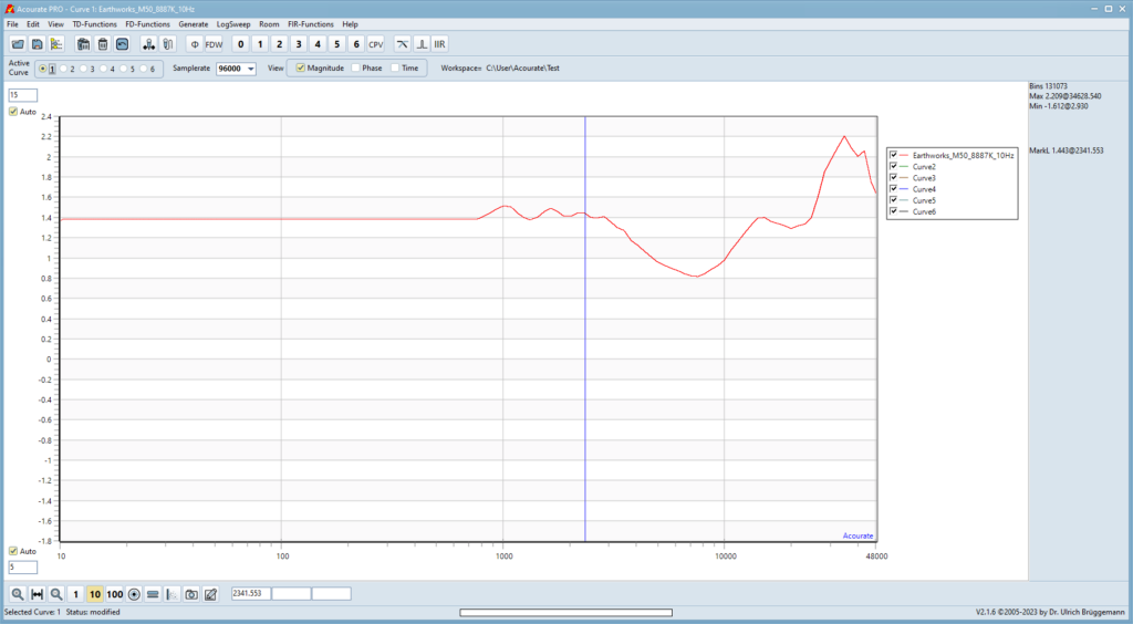
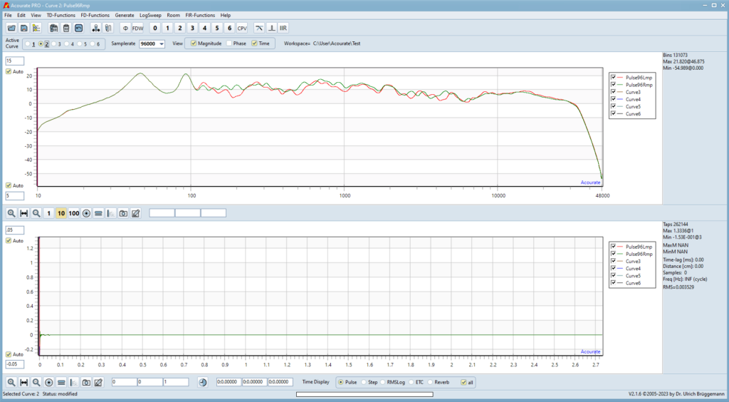
Acourate: Amplitude of my Earthworks M50
My curve reaches a minimum of 0.8dB and a maximum of 2.2dB. The average value is 1.4dB.
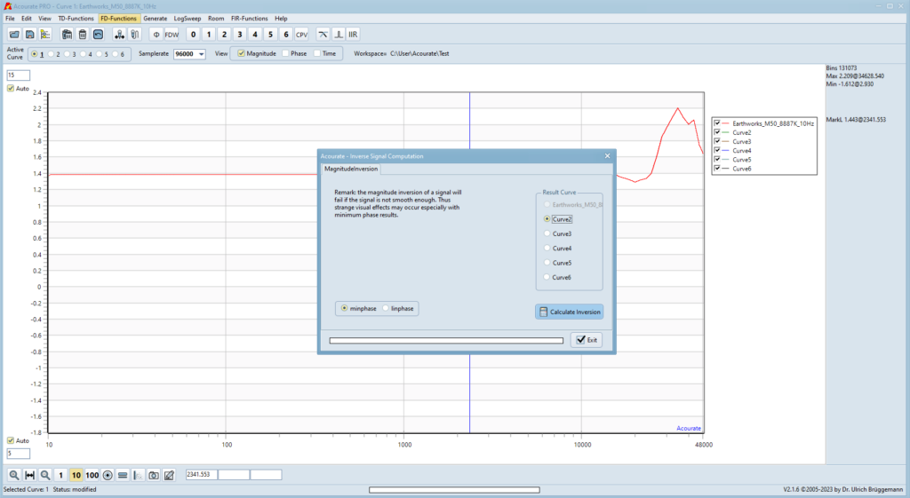
In my case, I now have to calculate the inverse from the data. By calling
FD-Function -> Magnitude Inversion
you will get the following window
Acourate: Inverse Signal Computation
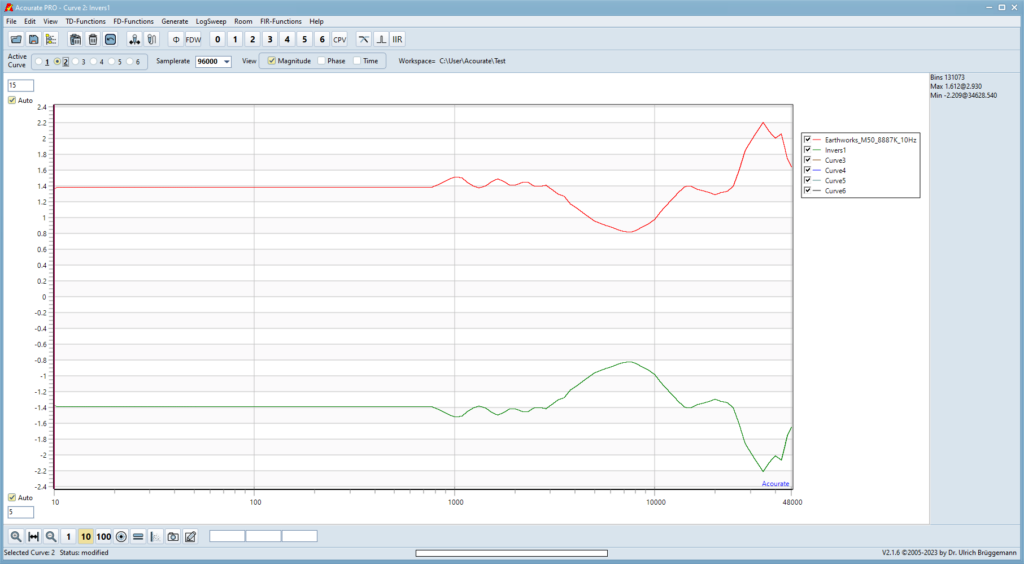
Here you select “minphase” and “Curve2”. The inverse is then calculated with “Calculate Inversion” and displayed in Active Curve 2.
Acourate: Amplitude & inverse amplitude of my M50
Finally, the inverse must be saved. This curve is used to linearize the measurement curve for all subsequent measurements. You must ensure that the Active Curve 2 window is active. With the menu item
File -> Save Mono WAV
the inverse is then saved. You must first decide on the format of this file (“desired resolution”). On a high-end system, the choice is naturally “64: double float (default)”. Finally, you can assign an individual name for the calibration file. In my case, the file is called “M50Invers96-262k.wav”. I can therefore take all the relevant information from the name.
If you have already received inverted data from the manufacturer, the inversion step is not necessary. After reading in the data, the curve is then saved with Active Curve 1 activated as described above.
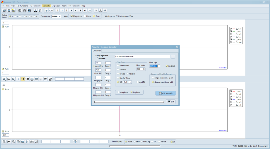
Generation of the Crossover
June 5, 2025
With a setup like mine, no measurements of the overall system can be carried out without a crossover running on the Acourate Convolver. Of course, the routing of the audio signals must have been performed successfully beforehand.
I have a separate folder with a number of subfolders for the crossover files. All possible experiments with the crossover are stored there. Again, I try to choose concise names. There is also a separate description for each calculation in my Joplin.
First, the folder for the crossover is defined as the working folder. The crossover is then created in Acourate with
Generate -> Crossover
All relevant parameters are specified in the window that opens.
Acourate: Creation of a Crossover
The parameters for my crossover have already been added. I use a 3-way crossover with crossover frequencies of 125Hz and 7.5kHz. I never use the delays at this point, a value of 0 is specified for all of them. I use UB jPol11 FIR filters with an order of 2 as the filter type (without dynLTA). As described above, I let the crossover calculate with the maximum possible number of taps (262144). The crossover is created with linear phase (linphase). The big advantage of FIR filters over IIR filters. The “double precision” file format is already preselected. The files are generated with “Calculate XO” and saved in the current directory.
A linear-phase (FIR) filter is described by
|H(f)| is the frequency response, ω is the angular frequency, and τ is the constant delay.
This means that all frequencies are delayed by exactly the same amount of time. This results in the following advantages:
no phase distortion
perfect transient response
perfect timing between the frequencies
A minimum-phase (IIR) filter, on the other hand, alters this phase. The result is
This means that different frequencies have different delays. The consequences are
Group delay distortions
Transients are minimally smoothed
However, linear-phase filters produce pre-ringing, which is not the case with minimum-phase filters.
dynLTA
Usually NT and UB crossovers do not show up a wide transition area between passband and stopband. So with a typical 3-way system just two crossovers max overlap for each frequency (imagine that with a 6 dB slope crossover multiple XOs can overlap in the same frequency range). Now it may happen that if two corner frequencies are too close together also with NT/UB three XOs share the same frequency range. At this point dynLTA gets into the game. With a preselected order of 1 you can mark the dynLTA option and Acourate will calculate the highest necessary filter order (floating point allowed) which is required to ensure that there are only two XOs sharing the same frequencies.
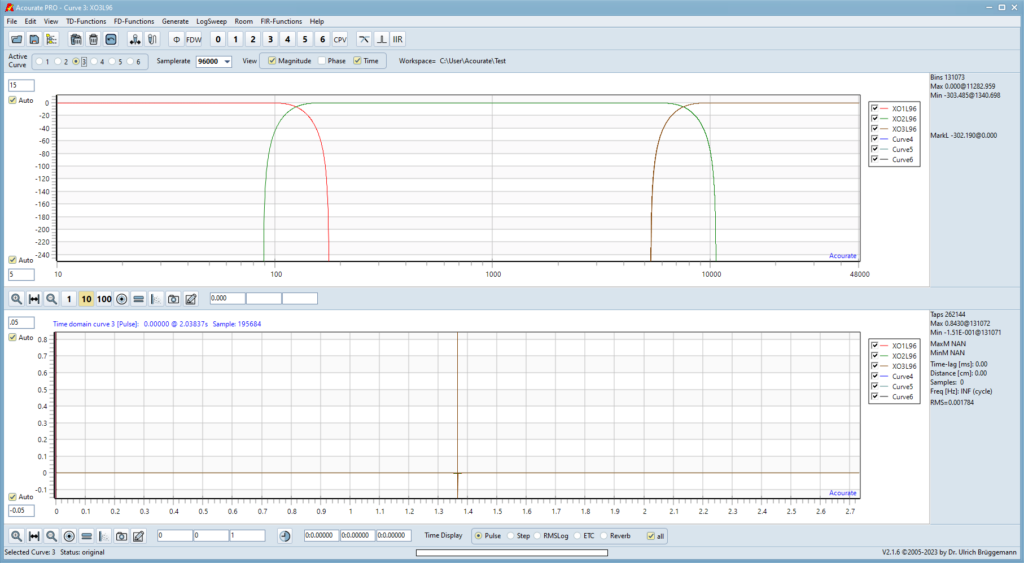
Acourate designates the crossover files as XO*.dbl. The numbering starts with the bass. L and R naturally refer to the left and right channels. At this point in time, the respective files of the two channels are identical. The number 96 provides information about the underlying sampling frequency.
Acourate: Left Channel of my 3-way Crossover
The picture above shows the frequency responses of the 3 ways for the left channel (top) and how they add up perfectly to a Dirac pulse (bottom). The crossover points in the crossover frequencies are at -6dB, exactly as they should be.
Finally, the generated files must be converted for the convolver. To do this, call
Room -> Create CPV for AcourateConvolver
Select the first entry in the selection window that opens. This is usually XO1L*.dbl, everything else then runs automatically. In addition to the *.dbl files, the corresponding *.cpv files can then also be found in the directory.
Special configuration for the RQM system:
In my RQM system, two 57 Quad ESLs run in parallel per channel. In terms of hardware, each Quad is controlled individually. So that I can also use individual correction files for each Quad, I create one with 2×4 XO files from the 3-way crossover.
I rename the XO3* files to XO4* and copy the XO2* files to XO3*. From Acourate ‘s point of view, this creates a 4-way crossover. However, at this point the XO2* and XO3* files are identical. My directory now contains the following files:
XO1L96.dbl, XO1R96.dbl – to 125Hz / RiPol Subwoofer
XO2L96.dbl, XO2R96.dbl – from 125Hz to 7,5kHz / upper Quads
XO3L96.dbl, XO3R96.dbl – from 125Hz to 7,5kHz / lower Quads
XO4L96.dbl, XO4R96.dbl – as of 7,5kHz / Mundorfs
Note: The fact that there are 2 identical frequency ranges per channel does not interfere with Acourate’ s final calculation of the correction files (see Macro 4).
Configuration of the AcourateConvolver
April 9, 2024
In the AcourateConvolver you can select 9 configurations, each with 3 filter banks. The corresponding convolution files (*.cpv) are stored in directories on the computer. However, I deviate from the location that is set up during the installation of AcourateConvolver and store all my data in a directory called
c:\conf
For me, this is the easiest way. But there is also no reason not to use the AcourateConvolver standard.
In this directory there are subdirectories with the names “1” to “9”. They refer to the total of 9 possible configurations. For each subdirectory, there are further directories with the names “1” to “3”, which are assigned to the filter banks. This is created during installation and I have adopted it in my directory. However, you can also create your own structure without any problems.
I always use configuration 9 for measuring and have labeled it accordingly in the AcourateConvolver. In the directory
c:\conf\9\1
I now save the crossover files created above.
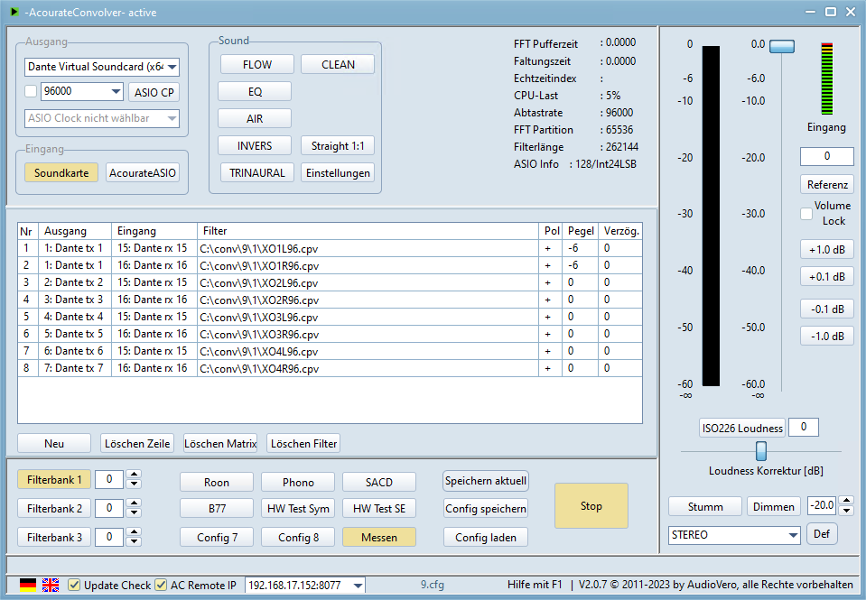
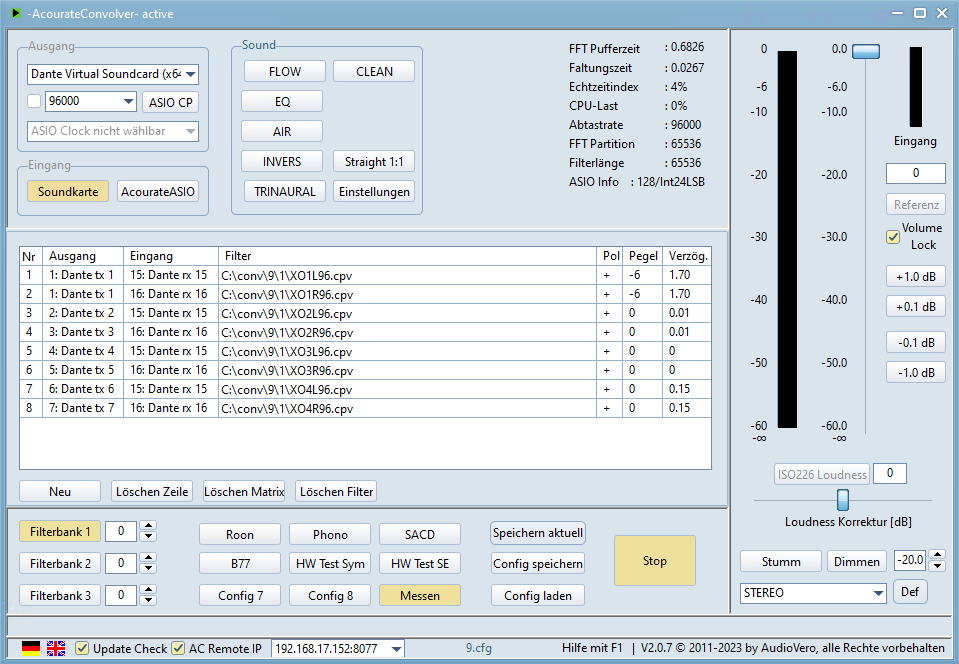
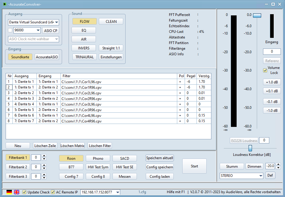
AcourateConvolver
The photo above shows the connection matrix as it is used in my system for measuring. The measurement signal from Acourate enters the convolver via Dante input channels 15 and 16. The audio channels for the speakers are routed to Dante outputs 1 to 7.
Here you can also see how to integrate a mono subwoofer. The signals from both bass channels (XO1*) are routed to output 1, but each with a level reduced by -6dB.
From this point on, the system is able to play reasonable sounds!
The AcourateConvolver is mathematically based on a convolution. It applies an impulse response h(t) to an input signal x(t) to generate a corrected output signal y(t):
Since the signals are digital – that is, discrete in time – the convolution is generated not by an integral but by a summation.
x[n] is the current audio sample, h[k] are the filter coefficients (impulse response), and M is the length of the filter.
For each new sample, the signal must be multiplied by the entire impulse response and summed.
With long filter coefficients, such as those used here, the computational load is immense. In the RQM system, with its 96kHz sampling rate and seven output channels, this results in 672000 samples (N) and thus more than 176 billion multiplications and additions per second! The number of arithmetic operations is calculated as follows:
The solution to this problem is the Fourier transform, since a convolution in the time domain corresponds to a multiplication in the frequency domain.
Even though the signal must be transformed twice, the approach using the Fourier transform is orders of magnitude faster. The following applies:
For the RQM system, the number of operations is reduced to just under four million per second. That’s a drastic reduction!
The convolver performs the following calculations:
The filter coefficients are available in the time domain and are transformed when playback begins. As a result, this FFT does not place any additional load on the processor during the ongoing processing of the audio signals.
the signal is transformed (FFT)
the two transformed signals are multiplied (Audio & Filter)
the result must be inverse transformed (IFFT)
Of course, there is also the additional time required to transmit the audio signals to the computer and output it again.
Position of the Measuring Microphone
April 9, 2024
The measuring microphone
should be reproducibly in the same position
should be positioned exactly in the middle between the two loudspeakers
for all measurements. The best thing to do is to devise a system for always placing the microphone in the same position.
My listening room has a wooden ceiling. With the help of my friend Heiner, I measured my listening position precisely with a cross-line laser and attached a hook to the ceiling at this position. I hang a plumb line on this hook with a mark at the correct height. This allows me to position the microphone pretty much exactly at the right spot in the room.
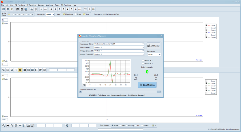
Then use Acourate and the “Microphone Alignment” function.
LogSweep -> Microphone Alignment
This allows the microphone to be brought into the center position with millimeter precision. The accuracy increases with the measuring frequency.
Acourate: Microphone Alignment
If you have positioned the microphone exactly in the middle, a green 0 appears in the window. The procedure is self-explanatory. With my type of alignment (see above), I only have to move the microphone a few millimeters to the left or right.
Higher Output in Mic Alignment
The mic alignment is based on the time alignment of tweeters.
It does not make sense to use e.g. subwoofers for the mic alignment as the timing of low frequencies is too slow. Thus the signal recorded by the mic will also contain reflections influencing the accuracy. Whereas high frequency signals should have more precise transients.
Thus the test signal for the mic alignment consists of Dirac pulses processed by a highpass > 4 kHz. The left channel contains two clicks, the right channel one click. This also means that the left channel sound a bit louder than the right channel. This is ok and intended.
As the clicks are quite short signal the playback volume needs to be increased.
The alignment function now records the clicks and tries to trigger on the incoming pulses. This should properly work if – the recorded signal has enough level (dependent on playback volume and mic gain) – the recorded signal detects a clear impulse (strong reflections should be avoided) – the tweeters have the same polarity (I have experienced the opposite several times even with „high-end“ speakers).
The alignment function then displays the recorded signal in the chart. In addition at the right side of the chart there is a number displaying the timing difference in samples, the target is to get 0. In addition there is an arrow pointing to the left or right direction as a hint in which direction to move the mic. If the arrow points to the left direction the mic should be moved left as the sound travel time from left speaker is longer than from the right speaker. I highly recommend to move the mic stand. This is more sensitive than moving/turning the mic itself. By the movement into the displayed direction the number must count down. If it counts up the left/right channels are switched.
The optimum is reached when the display is 0 and the chart shows two peaks without flat top.
The levels must be adjusted for a reasonable measurement. It shouldn’t be too “quiet”, but you shouldn’t overdrive either. For playback I use the volume setting on the preamplifier and for recording I use the gain factor of the microphone input on the Lynx converter.
The human ear has the greatest balance between frequencies at a sound pressure level between 80dB and 90dB. Mitch Barnett recommends an average measurement level of 83dB in his book. I have had good experiences with this and have calibrated my system to it when reproducing the measurement signals from Acourate. I use the inexpensive PeakTech 5055 sound level meter for this and set it to “C-weight / slow” for the measurement.
In REW, by the way, a level of 75dB is measured (see Check Levels). However, I have not had positive experiences with this lower level. I achieve better results with the 83dB specified above.
Since my system has very strong level fluctuations without optimization, I only carry out the measurement from 950Hz to 1050Hz with a duration of 60s. The sound level meter is held at the measuring position of the measuring microphone. I then set the volume control on my preamplifier so that I achieve approximately this level. There are also fluctuations in the narrow frequency range, I have to average “optically”.
Acourate: LogSweep Measurement
I measure with a level of 0dB in Acourate and -20dB at my preamplifier.
For those who do not want to afford a sound level meter or simply do not have one to hand at the moment, it is important not to set the level too low, but also not too loud. You have to rely on your own hearing. I also used this method for a long time for the basic setting.
With the playback level found, I then run a measurement over the entire frequency range and use it to set the level of the microphone preamp. In Acourate, the maximum measured input level is displayed on a green scroll bar (see below). This should not exceed -6dB. A dB up or down is not so important, but I make sure that I stay below this limit. It may be necessary to carry out this measurement twice.
Acourate: Input Level of the LogSweep Measurement
My microphone preamp is set to a level of 35dB for the Earthworks M50.
If nothing changes in the system configuration and the levels can be set reproducibly, this measurement only needs to be carried out once. Then always use the determined configuration.
Setting the Speaker Level
April 9, 2024
In a multi-way system, the speakers are connected to different power amplifiers. If they are not the same brand, it is very likely that the amplification factors will differ. In addition, the loudspeakers are also inherently different in volume.
It makes sense to match the levels of the speakers in the analog part of the system. In my system, this is particularly easy because I can apply a correction to each channel individually in the preamplifier. I make sure that my target curve is inserted as optimally as possible (see below). If you don’t take this step, Acourate has to take care of it. However, this can be at the expense of the digital “headroom” and there is a high probability of losing resolution.
I leave my Quads uncorrected, as they provide me with the basic level. However, I adjust the RiPol and the Mundorfs to the level of the Quads. One advantage of my solution in the VV7 is that I can not only attenuate but also amplify the individual levels. This means that the speakers can be corrected in both “directions”.
To determine the levels, start a measurement over the entire frequency range.
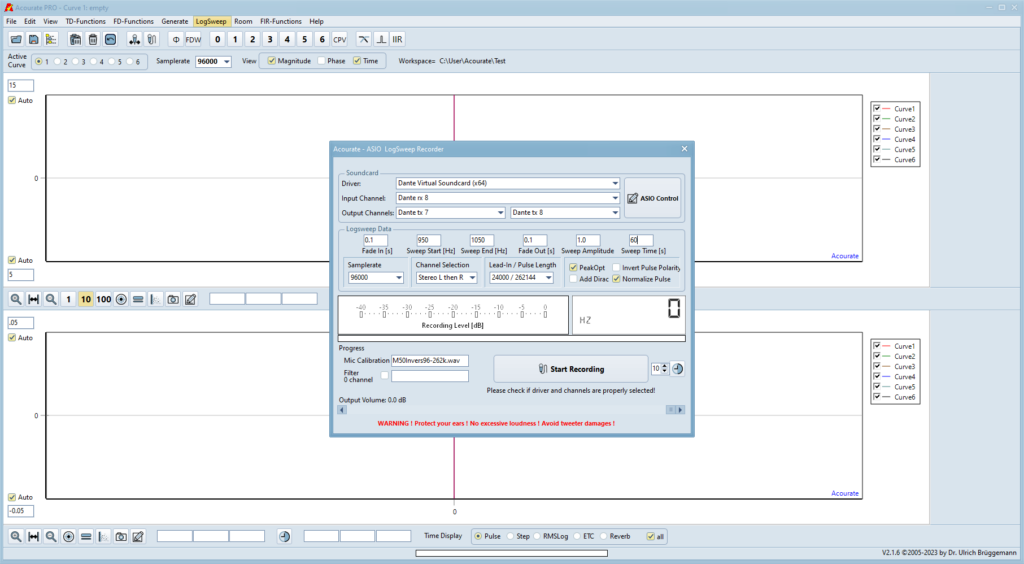
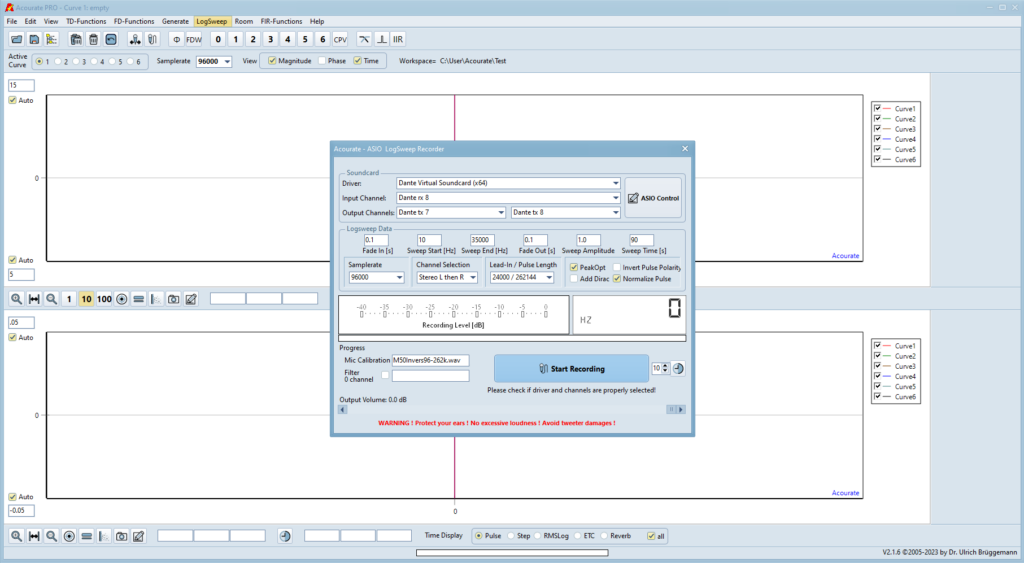
LogSweep -> LogSweep Recorder
This measurement does not have to be so precise. You can limit yourself to shorter measurement times. The result is then smoothed with macro 1. The output of the ICCC after the measurement can simply be acknowledged.
Room -> Macro 1
The parameters can be left at the default values.
Acourate: Room Macro 1
The following frequency response results for my system with the same output level at the preamplifier for all speakers.
Acourate: Uncorrected Levels of the Speakers in the RQM System
I took the picture above in macro 2 and also inserted my target curve (blue). This is the best way to see what I am writing about here. I will explain this further below. It is important at this point that the target curve is as high up as possible and that the actual signal does not fall below it at all.
I now made a volume correction of +5dB in the bass. The Mundorfs can remain at 0dB. After smoothing with macro 1 and calling up macro 2, I get the following results:
Acourate: Corrected Levels
After this setting, it may be necessary to adjust the measurement level again. However, this is not the case for me, as I only measured around 1kHz and did not change the level of the Quads.
Remark: At this point, I’m not really sure how you should adjust the levels. I have described my approach here. However, it will certainly also work if you make the two adjustments
Setting the Levels during Measurement
Setting the Speaker Level
in reverse order.
Time Alignment
April 9, 2024
One of the great advantages of a digital crossover is the ability to delay signals. This is used to correct the delay times of the individual speakers in a multi-way system so that they arrive at the listening position at the same time (time alignment). Acourate offers several options for determining the necessary delay times.
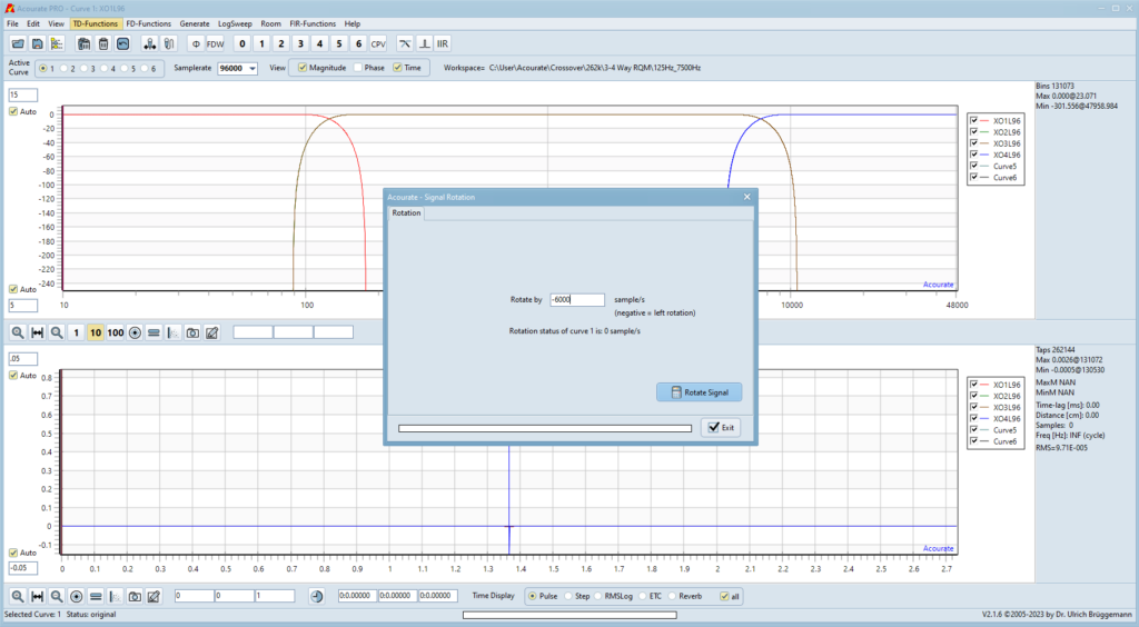
The procedure described here shifts the individual files of the crossover to each other in a defined manner. The tweeter (XO4*) is taken as a reference and left in its original state. The woofer (XO1*) is shifted by -6000 samples, the upper Quads (XO2*) by -2000 samples and the lower Quads (XO3*) by -4000 samples.
A negative value for the rotation shifts the signal forward in time, meaning that it is played back earlier. In the evaluation, the largest impulse comes from the tweeter and the smallest from the subwoofer. It is therefore necessary to move the subwoofer as far forward as possible in order to be able to clearly determine the impulse. At a sampling frequency of 96kHz, there should be 2000 samples between the individual drivers in order to be able to separate the individual impulses from each other in time.
Copy the crossover files created above (XO*.dbl) into a new directory. This is selected as the active working directory in Acourate. All curves that are still displayed (Active Curve *) should be deleted.
To do this, load the crossover files into curves 1 to 4. As the crossover files for the left and right channels are identical, it is sufficient to load only the files for one channel. The corresponding curves are then shifted and saved as left and right files.
TD Functions -> Rotation
The currently active curve is always moved using the “Signal Rotation” window.
Acourate: Rotate the Left Bass Channel
The newly created crossover files (*.dbl) must now be converted into *.cpv files.
Room -> Create CPV for AcourateConvolver
These are then transferred to the AcourateConvolver. I always use filter bank 2 in my measurement configuration for this. The files are therefore placed in the directory
c:\conf\9\2
Now select “Config 9” (Measure) and “Filterbank 2” in the AcourateConvolver. The matrix must then be configured and the setting saved. The Convolver is then started with this configuration.
Now it is time to carry out a first measurement in Acourate. The levels are set for this and the measurement microphone is in position and exactly centered (see above). With
LogSweep -> LogSweep Recorder
a measurement is started.
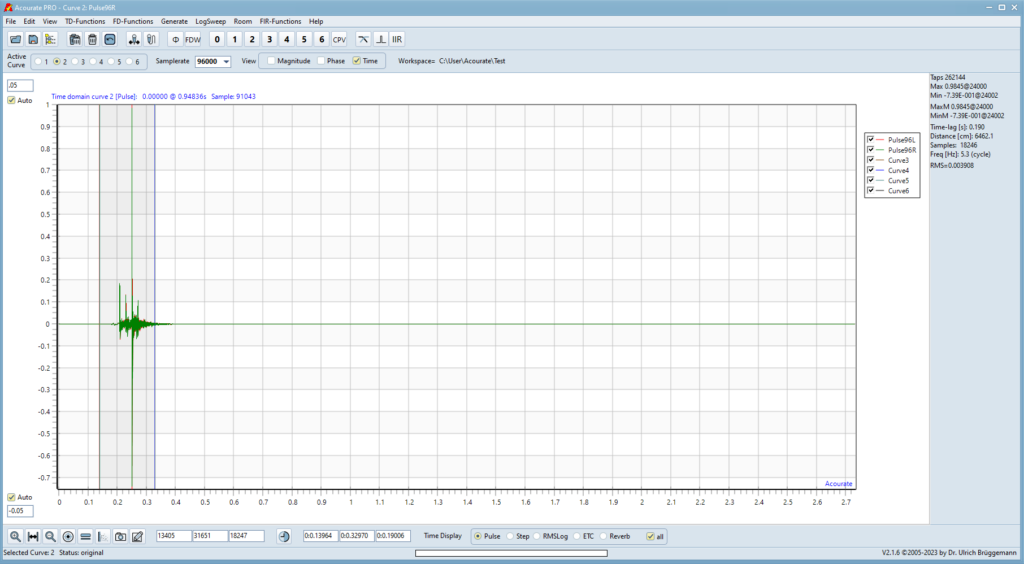
Acourate: LogSweep for Delay Time Measurement
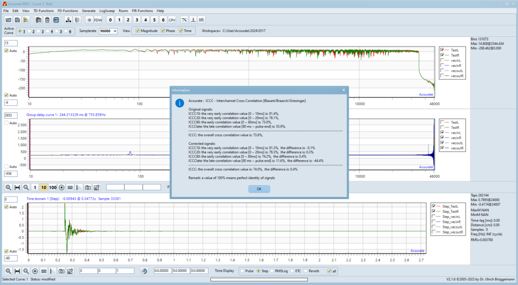
Nach der Messung erscheint erst einmal die Ausgabe für die Interchannel Cross Correlation (ICCC). Zum jetzigen Zeitpunkt kann man einfach auf „ok“ drücken und das Fenster schließen. Uns interessiert aktuell nur die zeitliche Auswertung der Messung. Aus diesem Grund kann man am oberen Bildschirmrand von Acourate außer „Time“ die beiden anderen Messwertausgaben deaktivieren.
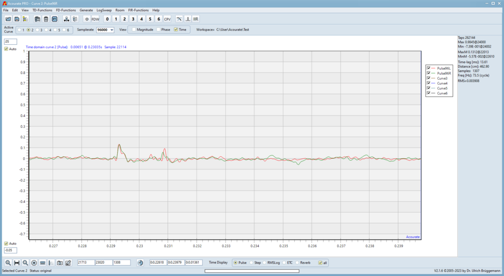
Acourate: Laufzeitmessung
The largest impulse is the tweeter, the two smaller ones in front of it are the midrange (upper and lower Quads) and barely recognizable, the small waves in front of it are the bass. If we had perfect timing between the individual loudspeakers, the impulses of the midrange would be exactly 2000 and 4000 samples before those of the treble and the bass would be 6000 samples before them. The deviations from this are the times we are looking for.
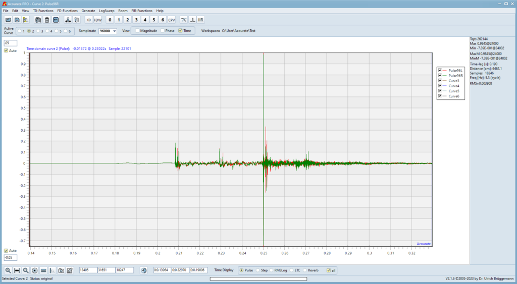
I carried out the measurement with 262144 taps (Pulse Length). This results in a lead-in of 24000 samples (see LogSweep above). Acourate displays the largest pulse precisely at this point.
Acourate: Runtime Measurement, Time zoomed
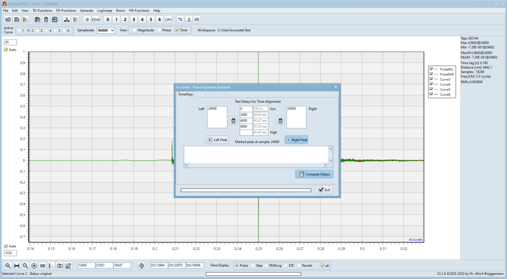
There is a clock icon below the time window at the center left. This opens the “Time Alignment Assistant”. However, there is a small peculiarity of my Acourate: you can only really open the Assistant once you have zoomed the signals in the Time window.
Acourate: Time Alignment Assistant
In “Test Delays for Time Alignment”, you enter the shifts made above – in this case 0, 2000, 4000 and 6000 samples. By clicking on “Left Peak” and “Right Peak”, the position (in samples) of the largest impulse in the “Left” and “Right” windows is adopted. As the complete signal is currently displayed, 24000 must appear on both sides.
The assistant is then exited with “Exit” and the measurement is zoomed so that only the pulse 2000 samples before the tweeter pulse can be seen. This corresponds to about 21ms, so the center of the displayed x-axis should be about 0.229s. There should not be a larger impulse at the edges of the display!
Acourate: Runtime Pulse at -2000 Samples
Now it’s back to the “Time Alignment Assistant”. Clicking on “Left Peak” and “Right Peak” again takes over the position of the currently largest displayed pulse. In my case it is 22013 in both channels. The deviation of 22000 samples is the desired time shift.
We now do the same for the two pulses around 0.208s (4000 samples).
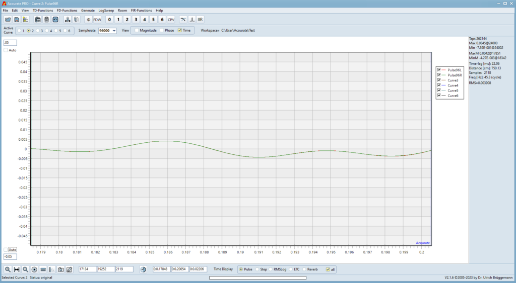
We continue with the bass impulse. Here, too, the area must first be zoomed accordingly. However, the bass impulse is very small and therefore difficult to recognize. But we know that it must be around 0.187s, 6000 samples before the high frequency pulse. In order to be able to recognize the pulse reasonably well, I have set the y-axis from “Auto” to ±0.05.
Acourate: Runtime Bass Puls
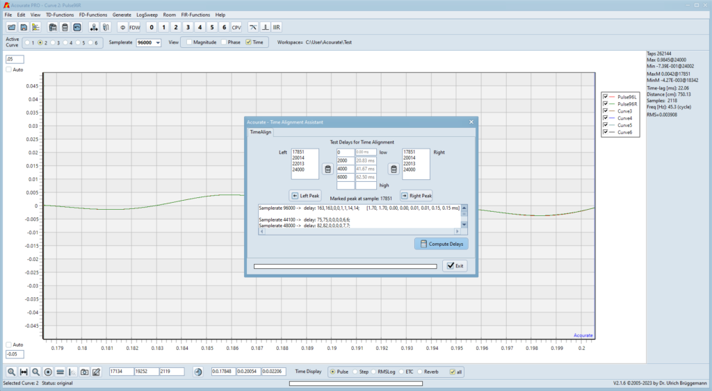
Now go to the Assistant one last time. The impulse is transferred to the left and right windows as usual. Then it’s time for the evaluation, which Acourate thankfully takes care of. Finally, click on “Compute Delays” to obtain the results:
Acourate: Evaluation of Runtime Measurement
We can see that the bass needs to be delayed by 1.70ms. The lower Quads are not delayed. The upper Quads are only delayed slightly by 0.01ms. The tweeters, on the other hand, must be delayed by 0.15ms compared to the lower Quads. These values are entered in the transfer matrix of the AcourateConvolver (Config 9 / Filterbank 1).
AcourateConvolver with entered Delay Times
The values are consistent, the mono subwoofer is in the middle and therefore closest to my listening position. The tweeters are also somewhat closer to the listening position. Consequently, these channels have to be delayed.
However, I had problems interpreting the values, so I took paper and pencil and did the math.
Calculation of the time delays from the determined values.
The pulse of the upper Quads starts at 22013 samples, but should start at 22000 samples. The pulse of the lower Quads starts at 20014 samples, but should start at 20000 samples. All four Quads therefore start too late. The low frequency impulse starts at 17851 samples, but should start at 18000 samples. The bass signal therefore comes too early.
First, the shifts in the signals are subtracted from the results – manually (TD Functions → Rotation) and by Acourate (24000):
Positive values therefore mean a delayed and negative values mean a premature reaction.
To correct the timing of the RQM system, the low frequency signal must be delayed by 149 samples and the signals from the Quads must be transmitted 13 or 14 samples earlier. However, it is not possible to play a signal earlier, as the system would have to be able to look into the future. Nevertheless, digital signals can be delayed very easily.
The solution is to additionally delay all speakers by the largest positive value of the samples determined above, in this case 14:
Now all time shifts are ≤0 samples. The signals therefore remain the same (0 samples) or must be delayed (<0 samples). This result can also be seen at the top of the “Time Alignment Assistant” window.
The biggest problem with this method is the very low bass impulse. In my case, detecting the maximum was still relatively easy. There are other speaker setups where this is impossible. Then you can use the method described in the Acourate Wiki (link – see above).
From this point onwards, we have a perfectly timed multi-way system!
Measuring the Speakers in the Room
April 10, 2024
We are now ready to measure the speakers in the room. To do this, a new directory is created and set as the active working directory in Acourate. All curves in Acourate are deleted. The microphone is in its measurement position, the levels on the preamplifier and microphone amplifier are set.
To be on the safe side, first check once again that the microphone really is exactly in the centre.
LogSweep -> Microphone Alignment
This is done quickly and ensures safety. If the microphone is not in the exact position, the measurement results are not really useful.
On the AcourateConvolver, the time-corrected crossover is running with Config 9 (Measure) / Filterbank 1 with the delay times entered.
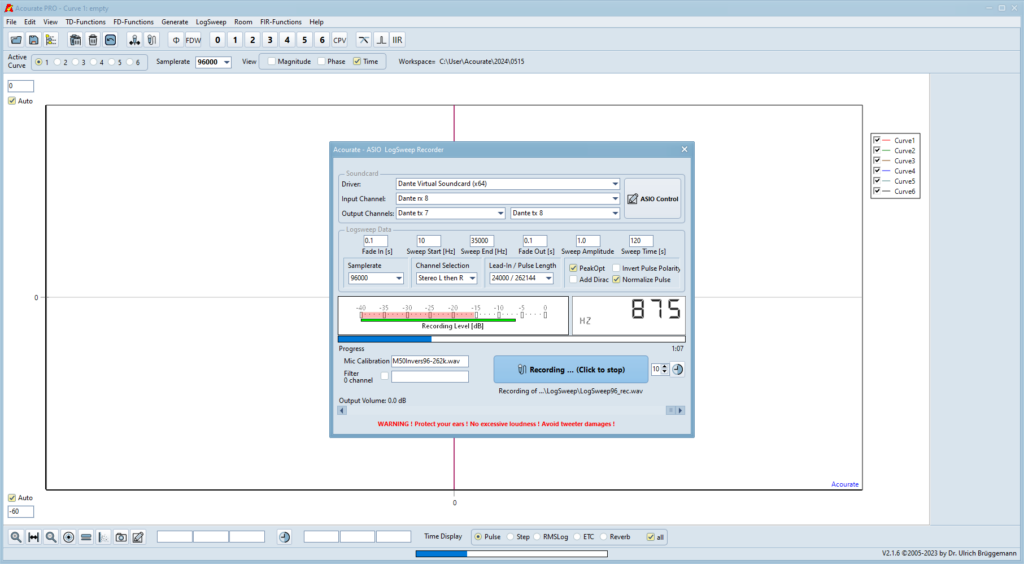
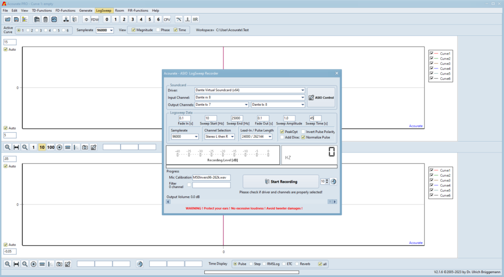
LogSweep -> LogSweep Recorder
You can remain in the room during the measurement, as you are also there while listening to the music. However, you should stand to one side. The triangle left loudspeaker – right loudspeaker – measuring microphone must be kept free.
Even in normal use, there is nothing between me and my speakers. According to Mitch Barnett, if you have a table or something similar standing there, for example, it makes sense to move it to the side. It obviously produces better results, even if the table is then put back in the same position. It’s definitely worth a try.
Acourate: LogSweep Measurement
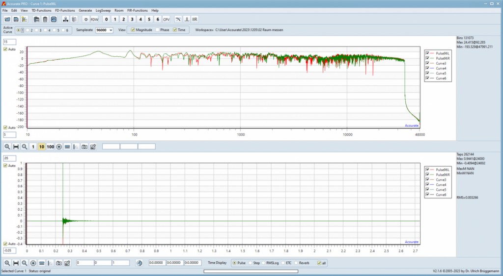
The measurement for one channel runs for 90s in my case. That’s quite a long time, but it increases the signal-to-noise ratio. I measure from 10Hz to 35kHz to get to the frequency limits of my speakers. For Lead-In / Pulse Length 24000 / 262144 is selected. The measurement is therefore carried out with the largest possible number of taps.
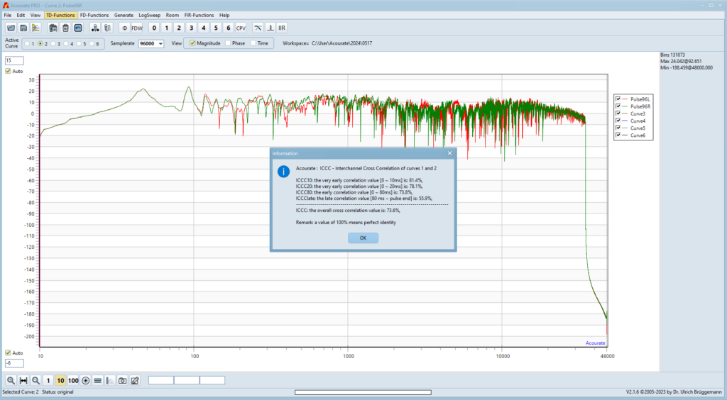
After the measurement, the window with the Interchannel Cross Correlation (ICCC) results appears (more on this below). At this point in time, you should simply acknowledge the issue.
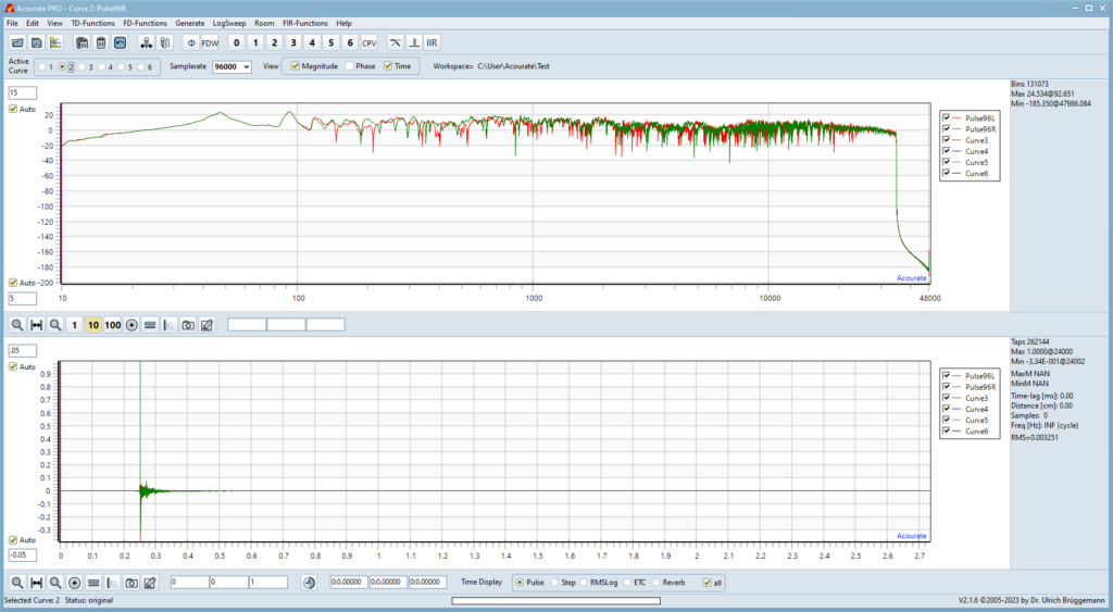
Acourate: Result of the Measurement
These measured values are now used to optimise the loudspeaker / room system. The measurements can be found in 2 files (Puls96L.dbl & Puls96R.dbl) in the current working directory. Acourate contains macros for further processing, which are processed below. These macros are extremely helpful and quickly lead to impressive results.
Room Macro 1 / Amplitude Preparation
July 3, 2026
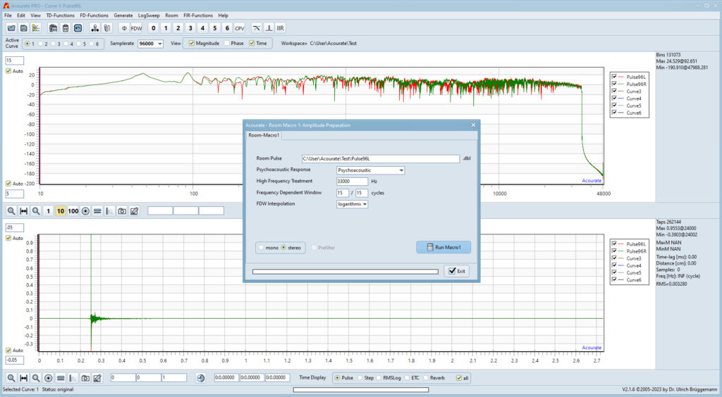
The pulse responses of the measurement must be processed first. They contain a lot of information that is not required for creating the correction filters. Using this macro, the frequency response is smoothed and only the first incoming signals are included in the further calculation by using a time window (FDW – Frequency Dependent Windowing). By calling
Room -> Macro1
the following input mask opens.
Acourate: Room Macro 1
The file specified under “Room Pulse” points to the measurement file of the left channel when called. There is usually nothing to select here.
With the “Psychoacoustic Response” selection menu, you can choose between “Psychoacoustic” and “Sliding 1/12-octave analysis”. It is recommended to leave the default setting. I have never tried anything else at this point.
With “High Frequency Treatment”, a frequency 1 or 2kHz below the maximum measurement frequency used should be entered. From this frequency, the signal is simply continued linearly during inversion (see below). Usually, a strong signal drop is obtained at the maximum measuring frequency. This is transformed into a sharp rise by the inversion, a behavior that we cannot tolerate. This signal behavior is prevented by this function. At that point, I specify a value 2kHz below the maximum measurement frequency, in this case 33kHz.
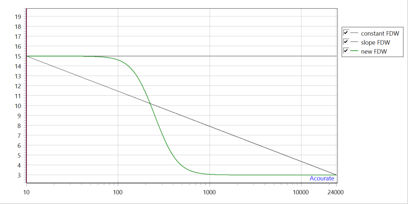
Selecting “Frequency Dependent Windowing” has a greater influence on the subsequent result. The two numbers are used to enter the length of the time window for averaging. The first value applies to the lowest and the second to the highest measured frequency. Acourate then adjusts the windowing between these two values evenly over the frequency curve.
I’ve experimented a lot with these settings. These days, however, I use the default values of 15/15.
Acourate Macro 1 FDW – What is meant by this?
The frequency-dependent windowing is defined in Acourate with a factor that specifies the window width not by direct time specification but by the number of frequency cycles. At 100 Hz, the cycle time is 10 ms. A factor of 5 therefore means a window width of 5 oscillations with 50 ms. At 10 kHz, this would be a window width of 0.5 ms. Within these 0.5 ms, just 1/20 of the cycle time of the 100 Hz is “swung”. Hence the window width as a function of the frequency. What comes after the window no longer plays any role.
Why do the entire thing at all: it’s not really about a smoothed frequency response curve, which is a by-product. You want to separate the direct sound from the room influences. At least from the late influences. What do I care what the room still emits in 1 second if the direct music event is important? It also makes no sense to correct something now so that it plays correctly the next day. This admittedly extreme approach simply shows that you are looking at the sound around the direct sound. If, on the other hand, the pure direct sound were treated, one would “merely” correct the loudspeaker and ignore the room with its often negative influences (e.g. room modes).
And so, when correcting the room, you are looking at a mixture of direct sound and room components. The FDW parameter allows you to control this. With the above example, you can look at e.g. 5 oscillations at each frequency and not, for example, 5 oscillations at 100 Hz and 500 oscillations at 10 kHz if the window width were constant across all frequencies.
The wider the window (or the higher the FDW factor), the more room component is included. With very large values, the listening position is logically more fixed because a change in the listening position also involves changes in the room component. The bottom line is: COMPROMISE, COMPROMISE, COMPROMISE! If you are the only listener (which is the case for many people) and your seat is fixed (sweet spot), you can make more corrections.
Acourate sets a default value of 15, but if you prefer, you can also use 3, 10, 25 or 12.7369. However, as the result also depends on the room, there is definitely no optimum value, only recommendations. It should be clear that at low frequencies the window width is greater than at high frequencies for the same FDW factor. Whether you increase the width at the bottom (10/5) or at the top (5/10) must be tried and tested for yourself.
Dr. Ulrich Brüggemann, 19 August 2024, Translated from the German forum aktives-hoeren.de
The last drop-down menu is “FDW Interpolation.” I always leave the setting there set to “logarithmic.”
Once all the parameters have been entered as required, press the “Run Macro1” button. Acourate calculates the smoothing and then outputs the result.
Acourate: Smoothed Amplitude Response
You can do more with the result than with the actual pulse response above. At this point you can see the uncorrected frequency response of the speakers in the room very clearly.
Partial Correction with FDW
Starting with Acourate version 3.3, there is an enhancement regarding the entry of FDW values in Macro 1. Although I do not currently have this version available, I would still like to mention it here. Therefore, here is a quote from the description:
Acourate V3.3 – Partial Correction and FDW
There is often debate over whether a “room” correction should correct the entire frequency range or only the lower range up to the somewhat mysterious Schröder frequency (see also Wikipedia).
Well, there’s another factor at play here, and in my opinion, it makes sense to consider them together. Inverting an original frequency response (which, incidentally, describes a steady-state condition, whereas music typically does not represent steady-state conditions) quickly leads to mathematical problems (aptly described as “ill-conditioned”). For this reason, frequency responses are often smoothed beforehand.
An excellent method for this is frequency-dependent windowing (FDW). It specifies which time interval is analyzed for a given frequency and is usually expressed in cycles. At 1kHz, the cycle time is 1ms, so 5 cycles define a window width of 5ms. At 20Hz, the window width is already 250ms. It’s easy to visualize this: just as in the example, the first 5 oscillations are used. Subsequent oscillations are suppressed. This method also allows for the evaluation of the important transient phase in the impulse response.
Now it makes sense to factor the speed of sound into our considerations. At 250ms, the sound has already traveled 85m, and by then there are already plenty of reflections (or, to use the fancy term, “sound reflections”) in the living room. At 5ms, the distance is just 1.7m — definitely a shorter sound path. This means that with FDW, at lower frequencies, more reflections are taken into account, and thus the room is factored in. Whereas at higher frequencies, the room is increasingly filtered out, and one is looking solely at the behavior of the speaker.
This leads to the realization that room correction is a combination of room and speaker correction. But what if the speaker is so good that I don’t want to correct it at all?
The 100% method involves simply smoothing the frequency response horizontally in the equalization above a selected frequency. This definitely works, but it still raises the issue of how to achieve a clean transition between the corrected and uncorrected regions. The level differences between the two regions must also be properly balanced.
The approach used in Acourate to date has been not only to specify a constant FDW across the entire frequency range, but also to allow users to specify two values — one FDW value for a lower frequency and a second FDW value for an upper frequency. A suitable value is then interpolated for each frequency in between.
This is shown here for a constant FDW 15/15 and an interpolated FDW 15/3 (black curves):
The latest version of Acourate, V3.3, now also allows you to specify a low-shelf profile. The graph now shows, with the green curve, an FDW profile that, at a cutoff frequency of 250 Hz and with a setting of 15/3, windows approximately 15 cycles down to 100 Hz and then, after the transition phase starting at 1 kHz, uses only 3 FDW cycles. The cutoff frequency and Q-factor are also selectable here; the lowest FDW value is 1 cycle.
As an example, here is the result of Macro1 + 2 for an arbitrary measurement result. FDW is 15 / 1. Corrections here occur primarily in the lower frequency range; in the upper range, there is essentially just a gentle left/right level adjustment.
Enjoy V3.3, and best regards.
Uli
Dr. Ulrich Brüggemann, May 26, 2026, Translated from the German forum aktives-hoeren.de
To use the new feature described above, select shelf profile from the FDW Interpolation drop-down menu.
When I look at the uncorrected frequency response of my RQM system and consider that my upper cutoff frequency isn’t until 7.5 kHz, I don’t see the point in correcting my system only in the lower frequency range.
However, I can certainly imagine that there are speakers for which such a correction would be effective.
However, you shouldn’t use this feature right away when you first start using Acourate on your own system. In my opinion, it’s more of a feature for experienced users.
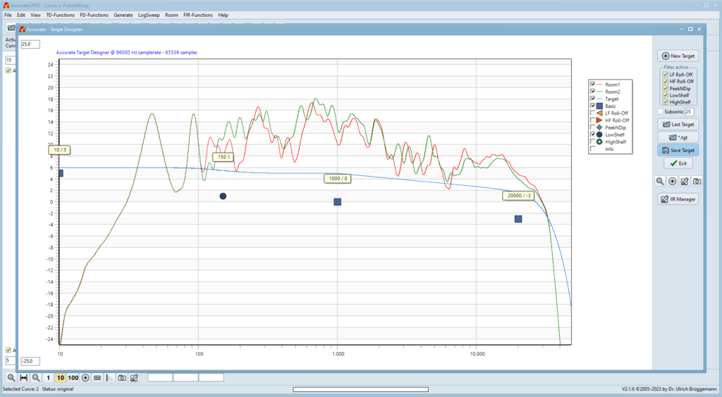
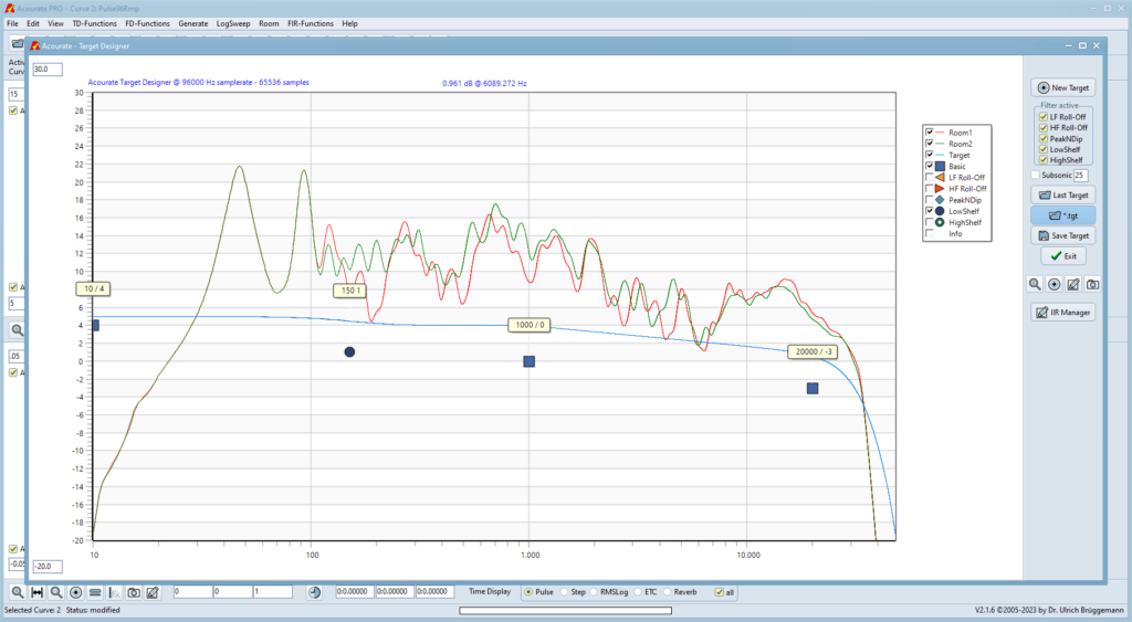
Room Macro 2 / Target Curve
April 10, 2024
This macro takes you to the crucial step of determining your own target curve. This curve is used to define the desired target frequency response of the system. There are many ways to determine this curve and you will want to try out a few things at first, at least that was the case for me. There is no such thing as an ideal target curve. It depends on the room, the speakers and your personal taste.
The companies Harman International and Brüel & Kjær have carried out research into an optimum target curve. You can quickly find the curves online if you search for them.
The recommendation for an initial curve is to start with a linear frequency response up to 1kHz (inflection point) and then drop the curve to -6dB at 20kHz.
This sounds very strange to a beginner, we audiophiles want to transmit our signals as uninfluenced as possible. My recommendation is to simply try it out, i.e. to select a target curve that simply runs linearly from the bass to the treble. That’s what I did, of course! After listening to a few notes of music with the resulting correction files, I quickly went back to the recommended curves. Believe me, nobody wants to listen to music like that.
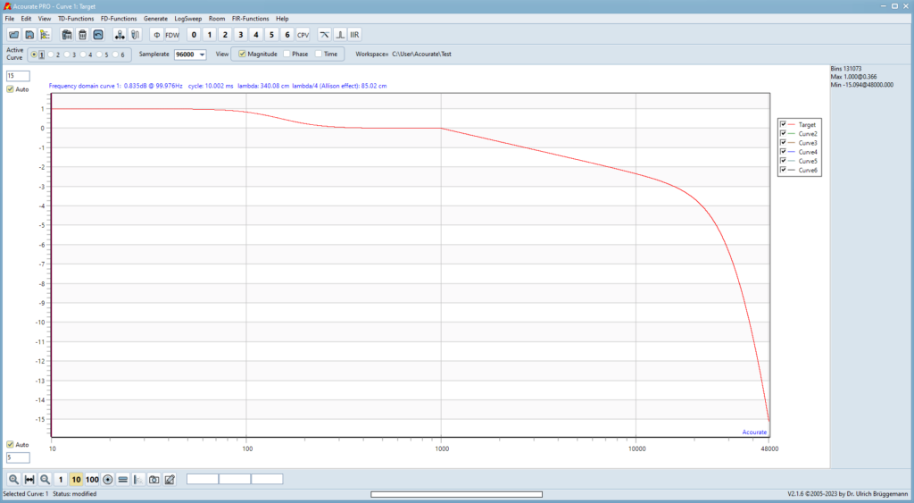
My target curve is linear up to 1kHz and then drops to -3dB at 20kHz. With highly directional loudspeakers it makes sense to attenuate the high frequencies less. There is also a bass boost (low shelf) of +1dB from 150Hz downwards. In addition, there is a low-pass filter at 30kHz. On the screenshot below you can see the course of my curve. I’ve been listening to it unchanged for more than a year now.
Acourate: My Target Curve
On the recommendation of Dr. Ulrich Brüggemann, you should not create a subsonic filter at this point. This is only done in Macro 4 (see below).
With the calling of
Room -> Macro2
it takes you to the Target Designer. Here you can create your own target curve using the graphical markers. A description of the functions and operation can be found in the Acourate Wiki.
I myself use the “Target.tgt” file. It is a text file that can be edited with any normal editor. If the text file exists from a previous optimisation, it can be loaded using the “*.tgt” button. It is generated by the Target Designer. As my target curve is defined, I only need to determine the base level of the curve in relation to the current measurements.
In the next section I show the relevant excerpts from my file. The upper values up to the “…” describe the recommended starting curve (see above) but with a -3dB cut at 20kHz. Below that you can see the low-pass filter and the low shelf. I am currently only adjusting the value for “0basicgain”.
Macro 2 also contains the “IIR Manager” button. In the window that opens, you can easily make the entries that I described in the previous sections. The diversions via a text editor is therefore not really necessary.
Acourate: Target Designer
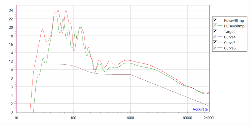
The picture above shows the position of my target curve (blue) in relation to the smoothed measurement results. The curve is shifted as high as possible without getting too many measured values below it. Only the measured values above the target curve are corrected. I accept a slight undercut at one point or another in favour of the digital headroom.
Once you are satisfied with the result, create the Target.dbl curve required for the calculations by pressing the “Save Target” button.
Acourate: Target Curve
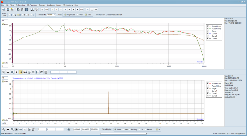
The target curve is displayed in Active Curve 3 after the calculations in the Target Designer.
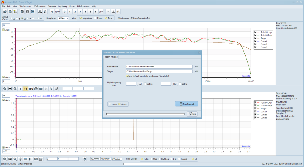
Room Macro 3 / Inverting
April 14, 2024
Before calculating the actual correction files, the smoothed measured values must be mirrored on the generated target curve. This is done by calling
Room -> Macro3
Basically, there is nothing to enter in the window that opens. The inverse curves are generated by pressing the “Run Macro3” button. The window closes automatically.
Acourate: Inverting
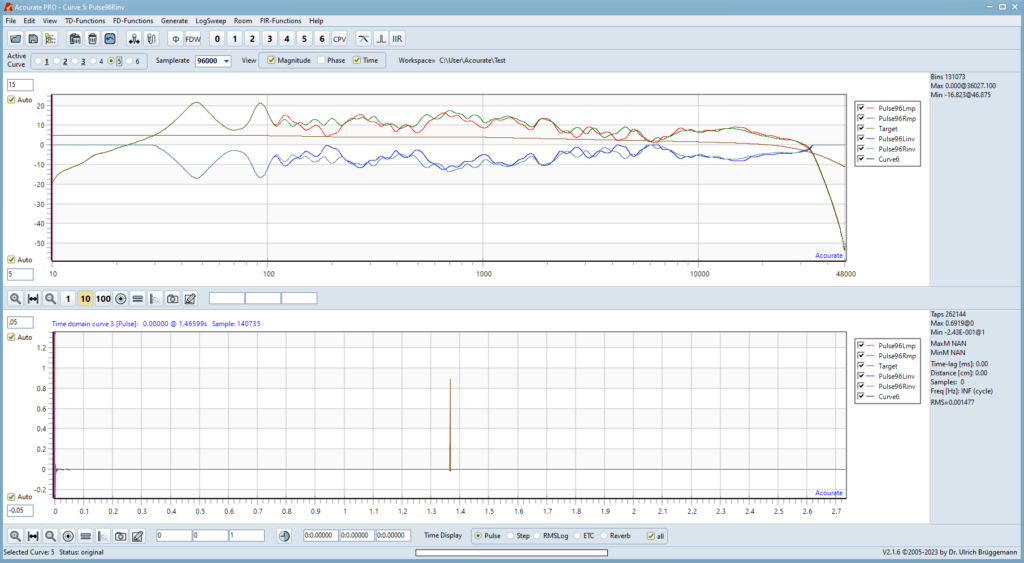
The smoothed measurement curves mirrored on the target curve are shown in Active Curve 4 and 5.
Acourate: Inverted Smoothed Measurement Curves
The frequency response of the inverses now also shows the effects of the “High Frequency Treatment” parameter from Macro1. From 33kHz, the original curves are no longer mirrored on the target curve; the signal is continued linearly. Otherwise there would be a steep rise in the inverse in the upper frequency range, the original curves drop sharply here.
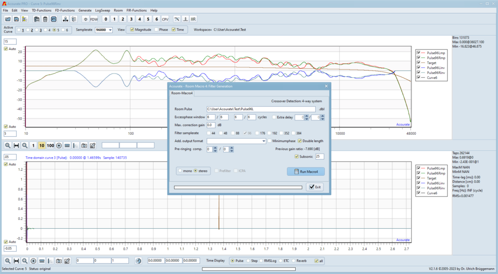
Room Macro 4 / Generation of Correction Files
April 14, 2024
Before you start calculating the correction files, you must ensure that the crossover files created above (XO*.dbl) are in the current working directory. This completes all the preparations. With
Room -> Macro4
opens the window for creating the correction files.
Acourate: Macro 4 / Filter Generation
The output “Crossover Detection: 4-way system” at the top right of the window indicates that the crossover files have been recognized. The information naturally refers to my RQM system.
Acourate: Macro 4 / Filter Generation
When entering the “Excessphase Window”, you should start with the default values for the first time. I have been using the values 5/5/5/5 for some time now. These parameters are similar to those in macro 1, but here you enter values for each channel individually. The first number again applies to the lowest and the second to the highest measured frequency.
I also select the “Subsonic” filter and enter a cut-off frequency of 25Hz. By the way, it is a 2nd order NT filter. I calculate the correction files with “Double length”. I leave all other parameters at their default values.
The correction curves are calculated with “Run Macro4” and then convolved with the crossover files. After the calculation, you will have the following files in the working directory:
Cor1L96.dbl, Cor1R96.dbl – to 125Hz / RiPol Subwoofer
Cor2L96.dbl, Cor2R96.dbl – from 125Hz to 7,5kHz / upper Quads
Cor3L96.dbl, Cor3R96.dbl – from 125Hz to 7,5kHz / lower Quads
Cor4L96.dbl, Cor4R96.dbl – from 7,5kHz / Mundorfs
We have now created the first correction files for the loudspeaker system and could transfer them to the AcourateConvolver after the corresponding conversion. However, you should first take a look at the result.
Room Macro 5 / Test Convolution
April 14, 2024
On the AudioVero homepage in the Infocenter under Instructions and Tutorials you can find the document:
Pre-ringing compensation (supplement)
It explains exactly what I will briefly describe below.
By calling
Room -> Macro5
a test calculation is carried out. The measured signals are calculated with the correction filters created. Without having to measure the corrected system, the behavior of the speakers with correction is obtained in this way. If you then check the system out of pure curiosity, you will be amazed at how congruent the two results are.
Acourate: Result of the Calculations from Macro 5
In the bottom window (Time / Step), you can see the oscillation before the actual step responses. You can try to reduce these with smaller values in the “Excessphase Window” (Macro 4) or even eliminate them completely, but you will pay for this with a lower phase correction. Nevertheless, this may be the right approach for your own system.
For me, on the other hand, the compensation of the pre-ringing has proven to be the right approach.
In the middle window (Phase / Group Delay), only the two input signals vecinL and vecinR are activated. You can recognize a peak (bell curve) at approx. 80Hz for both signals. The respective number of peaks in the right and left channels are counted, in my case it is one each. The very large peak at the right edge >30kHz is not taken into account.
This result (1/1) is used to return to macro 4.
As I mentioned above, a linear-phase filter is characterized by the fact that it shifts the phase of all frequencies by exactly the same amount. For this to work, the impulse response must be symmetric:
The filter’s main pulse is centered, so there is already energy present before it. This means that a short pulse produces a response that begins even before the pulse itself. This behavior is known as pre-ringing. It is related to the time-frequency duality of the Fourier transform and is therefore a purely mathematically generated effect.
Pre-ringing can be problematic. The human ear perceives time asymmetrically, since in nature there are no effects that occur before their cause.
Addendum
In mid-July 2026, I received Acourate version 3.3.3 with a note stating that the PRC in Macro 4 was no longer available. When I asked how I should compensate for the pre-ringing in the future, I was told to just give it a try. No sooner said than done… I used my latest measurements and performed the optimization from Macro 1 to Macro 4 with the new version as described above. When I checked with Macro 5, there was no pre-ringing at all.
I’m thrilled!
In this version, pre-ringing compensation appears to occur automatically. This is a very well-designed and helpful enhancement to the software!
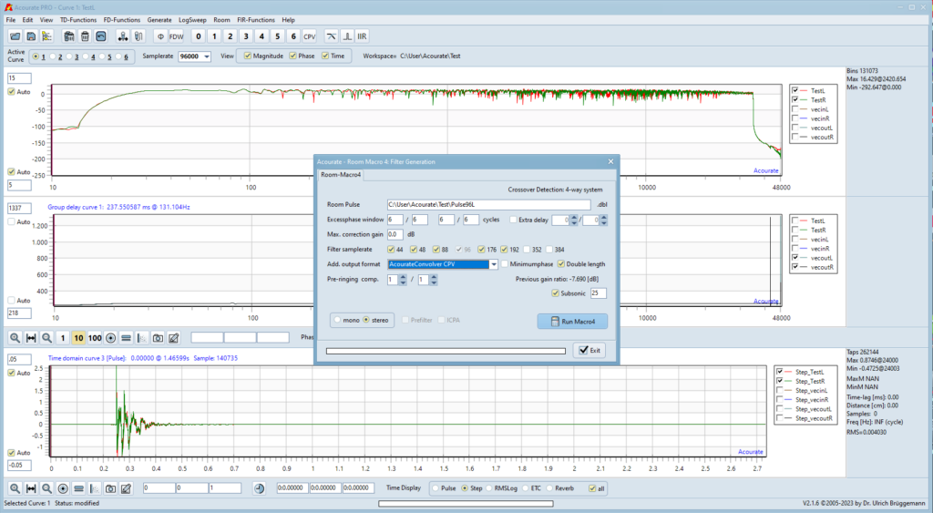
Room Macro 4 / Second Call
July 19, 2024
In the window of macro 4, the values just determined for the left and right channels are entered at “Pre-ringing comp”. At this point it is a 1 in each case.
Acourate: Macro 4 / Filter Generation
Note: Starting with Acourate version 3.3.3, this step is no longer included.
In addition, I now select all frequencies relevant for my converter under Filter samplerate. For my Lynx Aurora(n) these are 44…192kHz. I also enter the desired format of the correction files under Add. output format. For use with the AcourateConvolver, these are AcourateConvolver CPV files. The correction files can then be created with Run Macro4.
The result of the compensation can be viewed by calling macro 5 again. I will spare myself the presentation of the result at this point. I can report, however, that the ringing has disappeared in my constellation.
The cpv files generated in this way should now be transferred to the Convolver PC.
c:\conf\1\1
AcourateConvolver: Matrix with the final Correction Files
Above is the matrix of the AcourateConvolver for my RQM system, showing the corresponding entries.
Once you have reached this point, you can run your multi-way system with room correction. At this point, you should stop and live with the result for a while.
Room Macro 6 / Inter Channel Phase Alignment
June 12, 2024
To describe this feature of Acourate (from Ver. 2.0.0) I would like to use a small excerpt from the documentation:
ICPA – The Optimization of Unbalanced Stereo Setups
In room correction, each stereo channel is usually measured and amplitude and phase corrected separately. It has been shown that an additional improvement is possible if both channels are then considered together and optimized with regard to mutual interactions. This applies in particular to the modal frequency range up to 350Hz.
The cause is:
Asymmetry
Acourate V2 now offers an additional option to improve the listening result with suitable filters. These filters only influence the phase response over the frequency band, but not the amplitude frequency response. This means that the amplifiers do not have to provide more or less power. The indirect sound component also remains unchanged.
Acourate Documentation
This optimization is carried out after the first call of macro 4.
Once the correction filters have been calculated, the next step is to create symmetry between the two channels. Corrections are only made to the phase of the signals. In Acourate, this calculation is called Inter Channel Phase Alignment (ICPA) and is calculated with Macro 6. In addition, every user of version 2 has the document “ICPA – The optimization of unbalanced stereo setups” as a pdf file on the computer with Acourate.
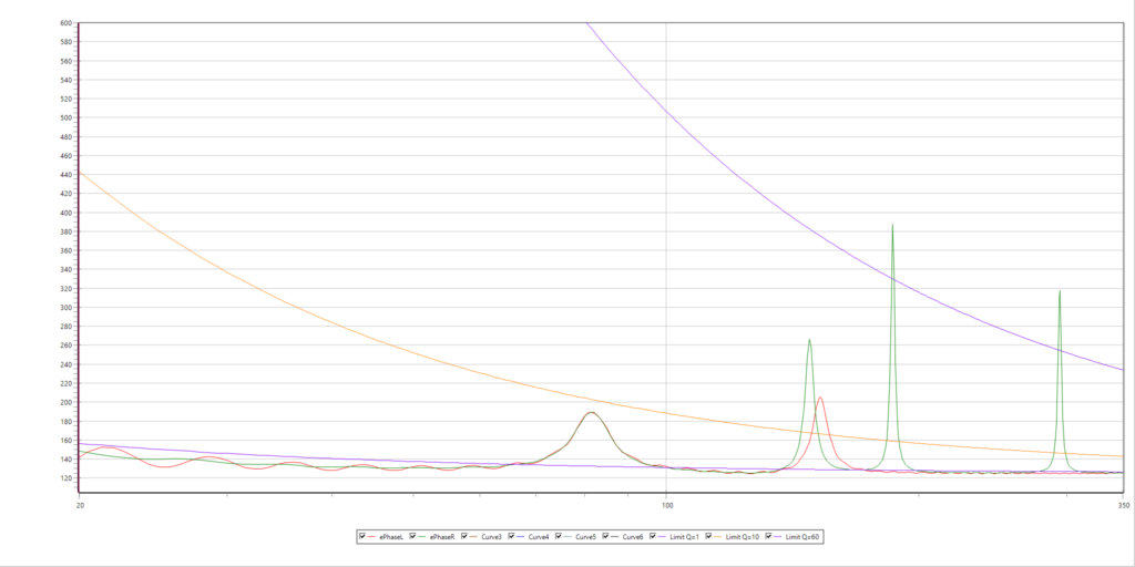
After the first execution of macro 4, macro 6 can be called. For the RQM system you get
Acourate: First Call of Macro 6 of the RQM System
The peaks below Q=10 (orange line) are compensated in their own channel. For the RQM system, these are the two peaks at approx. 81Hz. All peaks above Q=10, but below Q=60 (the purple line), are reproduced in the other channel. Here it is the peaks at 148Hz and 152Hz. All peaks greater than Q=60 remain uncorrected.
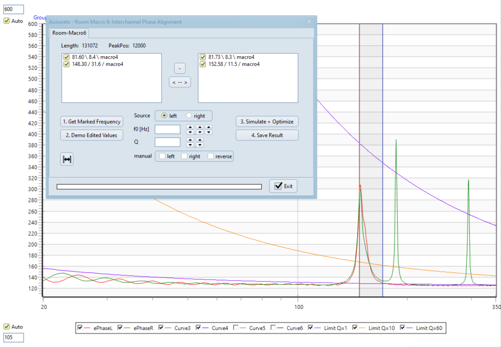
I have gotten into the habit of compensating for a peak and then running Macro 4 again. After calling up macro 6 again, you can then see directly how well the peak has been compensated or reproduced. Then I move on to the next peak …
To determine this, it is best to first zoom in on the peak to be processed and then place the marker on the peak. Do not forget to select the correct channel under “Source”. Use “1. Get Marked Frequency” to transfer the values to “f0 [Hz]” and “Q”. These values can then be changed using the arrow buttons. Click on “2. Demo Edited Values” to display the modified curve. If you are satisfied with the result, click on “3. Simulate + Optimize”. You can then see how the setting affects the phase. If you are satisfied with the correction, click on “4. Save Result” to save it. The setting appears in one of the two upper windows. If the results are marked with “/ macro4”, they have already been calculated with this macro. Macro 6 is exited by clicking on “Exit”, but the corrections determined up to that point are not lost.
Acourate: Macro 6 with Corrected Peaks
The picture above was taken after determining all 4 peaks relevant for the RQM system. The compensation at 81Hz works perfectly, the reproductions at approx. 150Hz quite reasonably.
Finally, macro 4 is called again. This time, however, the additional frequencies and the *.cpv files are generated (see: Room Macro 4 / Second Call).
Acourate sets the checkmark in front of “ICPA” if it finds corresponding results in the current working directory. This means that the ICPA results are included in the correction files. If you do not want this, you can also remove the tick in front of “ICPA”.
Reverberation Time
June 19, 2024
The reverberation time is the time interval within which the sound pressure in a room drops to a fixed fraction of its initial value when the sound source suddenly stops (reverberation). In most cases, one thousandth is used as a fraction, which corresponds to a decrease in the sound pressure level of 60 dB. The corresponding reverberation time is then referred to as T60 or simply T, usually as reverberation time (RT). It is one of the best-known key figures in room acoustics.
…
In 1898, the American physicist Wallace Clement Sabine discovered through experiments that the reverberation time is proportional to the volume V of a room and inversely proportional to the equivalent absorption area A of the surrounding surfaces, i.e. the larger the room and the more reverberant (reflective) the surface materials, the longer the reverberation time:
k is a proportionality constant with the unit s/m.
As I wrote in the introduction, the first measurement in my room led to the development of the active absorber. This measurement showed that my room has too long a reverberation time below approx. 70Hz. The absorber removes excess energy from the room in a defined way. In a domestic listening room, these problems only occur in the bass range below the Schröder frequency (approx. 300Hz).
Room Modes
Below the Schröder frequency, acoustic modes in the room can cause perceptible sound colouration. As these particularly affect the low tones, they are perceived as booming or one-note bass. Above this frequency, on the other hand, they do not cause any audible distortion of the reproduction in living rooms because the modes merge into one another in the form of dense reflections and reverberation.
If you have a LogSweep measurement available (see Measuring the Speakers in the Room), you can determine the reverberation time of the room directly from this. By selecting
TD-Functions -> RT60: Reverberation Time
you can access the evaluation. At the top right, you must first enter the standard for which the evaluation is to be calculated. For audio playback, this is “DIN 18041 Music”. Below this, enter the size of your room. My room is classically rectangular, so I have no problems with the input. Ultimately, however, it all comes down to the room volume (see citation above) and so you can also enter values that don’t quite correspond to reality but lead to the correct volume. You can also use the “+ correct” input field for this. I have already practiced this successfully with various non-rectangular rooms.
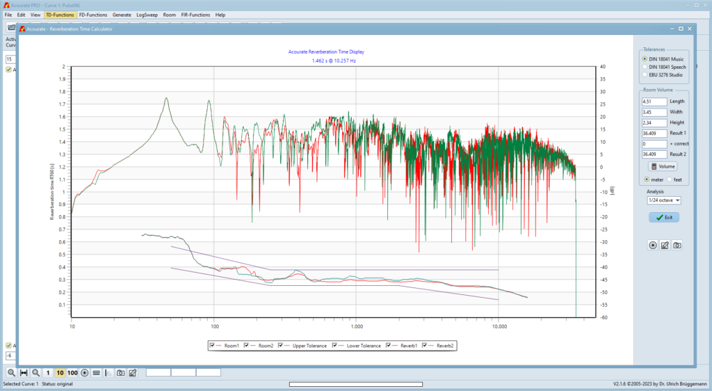
Acourate: Measurement of the Reverberation Time
The measurement above shows the reverberation time in my listening room with the absorber switched off. The shaded lines show the range in which the reverberation time should be for the standard and the volume entered. I don’t find downward deviations disturbing, as they make the reproduction even drier. Deviations upwards are clearly perceptible as booming.
As you can see, there is a problem below approx. 70Hz. It may not look very serious, but the trained ear will immediately hear the blurred and imprecise bass information. Once you have become familiar with a correct reverberation time, there is no way you can live with this result!
I use this measurement to optimize the settings of the active absorber for my room. Over the years, we have developed a set procedure for this, but fine-tuning involves varying the parameters and then measuring the effect. It’s a little time-consuming, but the result justifies the time invested.
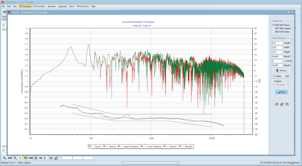
Acourate: Measurement of the Reverberation Time
The measurement above shows the situation with active absorber and optimized parameters.
This is how it should be!
Unfortunately, it is impossible to describe verbally what the curve above really means. You have to hear it and then understand what you are hearing.
To make it very clear once again at this point: The reverberation time is purely a function of the room! The most effective way to reduce excessive reverberation time is to use an absorber. This does not always have to be an active (electronic) solution. If you like working with wood and would like to work on this topic, you should take a look online under the keyword Helmholtz Resonator.
For the sake of simplicity, I have borrowed the following text passages from the Acourate Wiki.
IACC Interaural Coherence Coefficient
In this evaluation, the signals of the left and right channels are compared with each other within different time windows. This allows conclusions to be drawn about the quality of the stereo image. These are influenced by the speakers themselves (pair matching) as well as by the acoustics of the room. Both the positioning of the speakers and acoustic measures can be optimized by comparing the ICCC.
IACC10: The incoming sound in the first 10ms should preferably reach a value above 80% for good stereo imaging. Speakers with a high degree of directivity achieve high values here due to their design.
IACC20: The incoming sound in the first 20ms consists of direct sound and the first incoming diffuse sound. For stereo imaging, early reflections in the first 20ms should be avoided. If these arrive differently from the left and right channels, the ICCC value is reduced. If these are recognized and eliminated by suitable acoustic measures, the ICCC values increase.
IACC80: The sound in the first 80ms contains much more spatial information than the previous two values.
IACClate: Compares the reverberation produced by the two channels.
Remark: In the meantime, the function has been renamed ICCC – Interchannel Cross Correlation.
It should also be noted that the channels for ICCClate should not be correlated and so the value should be as small as possible. The ICCC overall cross correlation is in the range of 65…75% for most good audio systems.
At the moment, I have only installed two acoustic treatments in the room in addition to the active absorber. A curtain made of stage molleton hangs partially in front of the window and the door is covered with heavy foil (see: reverberation time). It is practically impossible to rearrange the furniture or speakers in the room. So I have to live with the circumstances. However, I have been planning to use diffusors on the wall behind the loudspeakers for a long time …
Acourate: ICCC after Optimization
Above you can see my result after optimization by Acourate. ICCC10 has deteriorated slightly. ICCC20 and ICCC80, on the other hand, have improved a little. There has been a drastic change for the better with ICCClate. The ICCC mean value improved from 73.6% to 74.0%. Basically, I can be quite satisfied with the result. But there is still a lot to do (see ETC)!
However, you should not be overly influenced by the figures. They show you whether there is room for improvement in the structure of your own system (keywords: channel equality, initial reflections). Ultimately, however, everyone decides for themselves whether they are satisfied with the playback quality achieved.
In April 2026, I installed diffusers in my listening room. Since these transform the incoming sound waves into a broadband diffuse field, this inevitably leads to a deterioration in the ICCC values. I lose about 7% compared to the values shown above. Nevertheless, the audiophile benefit provided by the diffusers is quite remarkable.
Energy Time Curve
August 10, 2024
The Energy Time Curve (ETC) is used to measure the decay of an impulse over time in a room. Our perception of location is based on the direct sound and the first 20ms after it reaches our ears. The first wavefront should arrive coherently in time (keyword: time alignment). In order to avoid false room information, the early reflections must be suppressed or redirected.
If a speaker is located near a side wall that has a reverberant surface, it is possible that the reflected sound will have approximately the same level as the direct sound. This could not only influence the frequency response, but also affect the perception of the room information in the recording.
I have taken the following information from Mitch Barnett’s book: The Energy Time Curve plots the reflection threshold in dB relative to the direct sound against the relative delay in milliseconds. According to Toole (1990, Loudspeakers and Rooms for Stereophonic Sound Reproduction), the level of the reflections should be -15dB below that of the direct sound within the first 20ms. However, there is also the Technical Note EBU-Tech 3276 (Listening conditions for the assessment of sound program material: monophonic and two-channel stereophonic), which only requires -10dB here. And then there is the LEDE specification, which even prescribes a reduction of -20dB.
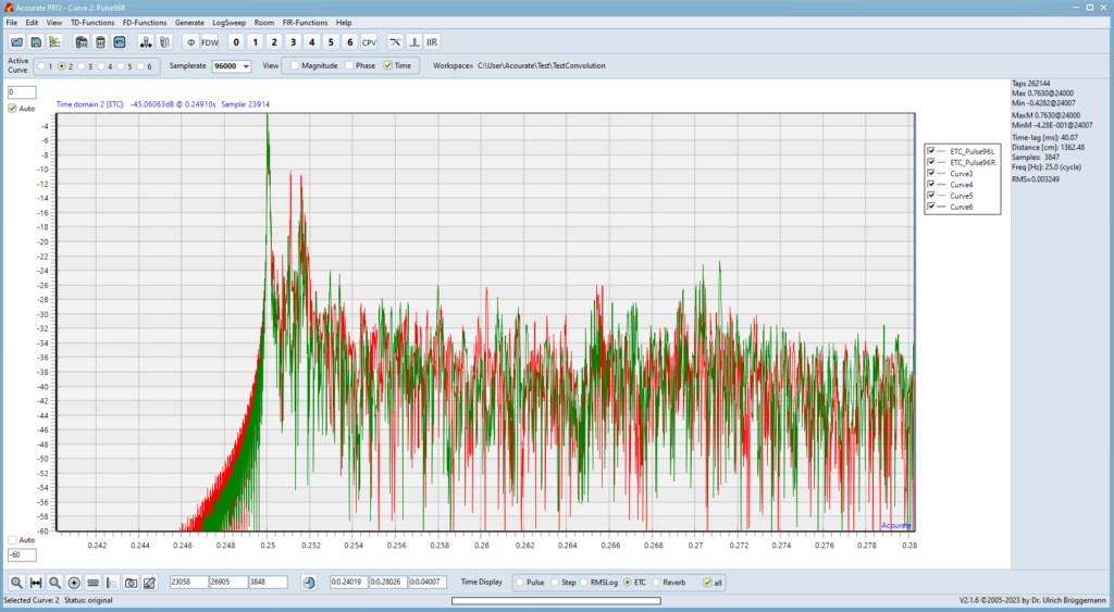
The ETC curve is obtained from a LogSweep measurement (see Measuring the Speakers in the Room). To do this, simply select the time window (Time) at the top of the screen and select the ETC option underneath the graphical display. The image below shows the result for a test convolution after optimization for my room.
Acourate: Energy Time Curve
In order to be able to make a better assessment, I have limited the y-axis to -60dB at the bottom. In addition, the signals are zoomed in time so that after the main impulse (0.25s / 24000 samples) only a little more than 20ms are displayed.
You can see that I have just met the EBU-Tech 3276 with -10dB.
My aim is to achieve at least the average of the three requirements, i.e. an attenuation of -15dB in both channels. But first I have to find out where the early reflections are coming from.
This is indicated by the time interval between the reflections and the main pulse at 0.25s (tP0). In the left channel there are 3 peaks above -15dB. There is only one in the right channel.
At a speed of sound of cS = 343m/s, the additional distances l of the reflections are calculated from
I measured the following times of the reflections in the left channel
and in the right channel
You can now use this information to calculate the additional distances that the reflections have to cover.
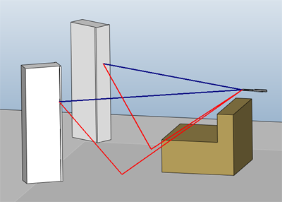
Recognition of disturbing spatial reflections in the pulse response
Once you have measured the distance that the sound additionally requires, the cause can be determined as follows: Stretch a string from the tweeter of the loudspeaker to the listening position, lengthen the string by the specified distance and determine which areas can be touched with the string: The Blue line is the path of direct sound from the speaker to the measuring microphone. The red line is the longer path of the diffuse sound. Instead of a cord, using a laser range finder is helpful. This way, even reflection points from the ceiling of the listening room can be measured easily.
As stated in the quote above, the reflection points are determined based on the tweeter. However, with my Mundorfs, there are no such reflection points at the calculated distance. This immediately raises the question of where to start when determining these points for a full-range driver. The two upper Quad panels can be ruled out right away. There are no suitable reflection points for them either, no matter where on the midrange/tweeter diaphragm I start. So only the two lower Quads remain. With them, there is the floor, which would fit the calculations. At least if one starts from the lower part of the diaphragm.