The RQM Loudspeaker System

Table of Contents

Introduction

19-03-2022

In the early 1980s I had the pleasure of listening to Mark Levinson’s famous HQD system. This system was an active three-way system with loudspeaker components from Hartley, Quad and Decca. For each channel, two Quad ESL 57s, arranged one above the other in a stand, were used, which reproduced frequencies from 100Hz to 7kHz. The frequencies above 7kHz were transmitted by a Decca ribbon tweeter modified by ML (without horn) and placed between the Quads. Two 24″ Hartley subwoofer systems were responsible for the low frequencies. Other components of the system included the ML LNC-2 active mono crossovers and the ML-2 Class A power amplifiers.

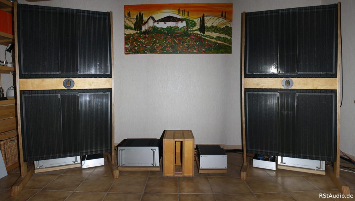
This listening experience left a lasting impression on me, especially since I was already the owner of Stacked Quads at that time. When I started building the subwoofer in 2008, it was clear to me that I wanted to build my own implementation of the HQD system. The result is an RQM system with the following components:

  • RiPol Subwoofer with a frequency range up to 125Hz
  • Quad ESL 57 in a stacked configuration, frequency range 125Hz to 7.5kHz
  • Mundorf AMT 1908C for frequencies above 7.5 kHz

Unlike the original system, I use a mono subwoofer, but it is more than sufficient for my small listening room.

The frequencies are split by the Lynx converter in conjunction with the Convolver PC, FIR filters are used. The Quads are driven by two ES4s (XA30.8 replicas) and the Mundorfs by an ES2 (Aleph J replica). The RiPol is powered by the ES3 as before.

Stacked Quads & Mundorf AMT

18-03-2022

With the original HQD system, the two Quads including the Decca ribbon can be rotated around the centre of the loudspeaker assembly – similar to an old school blackboard. In contrast to this, my RQM system has fixed stands, which has proven itself over the years (see Stacked Quads). The dimensions of the setup are such that the centre of the tweeter is 1m above the floor, which is pretty much the same height as my ears. The height of the baffle of the AMT is 110mm, just enough to mount this tweeter properly.

The frames are much more stable than the old ones. The whole structure can hardly be moved at the top – at the maximum lever. This not only gives you a good feeling, it is also clearly noticeable in terms of sound. The reproduction in the upper bass range has become even more precise, which speaks against the “school board” construction of the original HQD system. As a consequence, the stands will be supported against the rear wall with struts. This should remove any tendency to vibrate from the system. A solution that has been on my mind for a long time. The stands are already prepared for this.

One Stand of the RQM-Systems

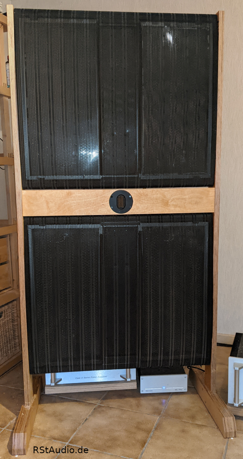
The stands are handmade in the usual perfect way by my friend Jürgen.
Dear Jürgen, I would like to take this opportunity to thank you once again for this wonderful work!

This is a combination of a planar radiator with a point source driver. The crossover frequency is critical and must not be chosen too low. I have made tests with 5kHz and 6kHz, both crossover frequencies are unusable. Especially at 5kHz the different radiation behaviour is clearly audible.

From my tests it is clear that the Mark Levinson people have made a wise choice with 7kHz. From this crossover frequency on, the different behaviour fades into the background. The AMT “only” transmits the harmonics of all significant musical instruments and supports the Quad in this range. In the end, I decided on a slightly higher crossover frequency at 7.5kHz. With this, the drivers form a very good symbiosis.

RiPol

19-03-2022

All information about the RiPol’s construction can be found on my page about this truly exceptional subwoofer.

View of the RiPol from diagonally in front

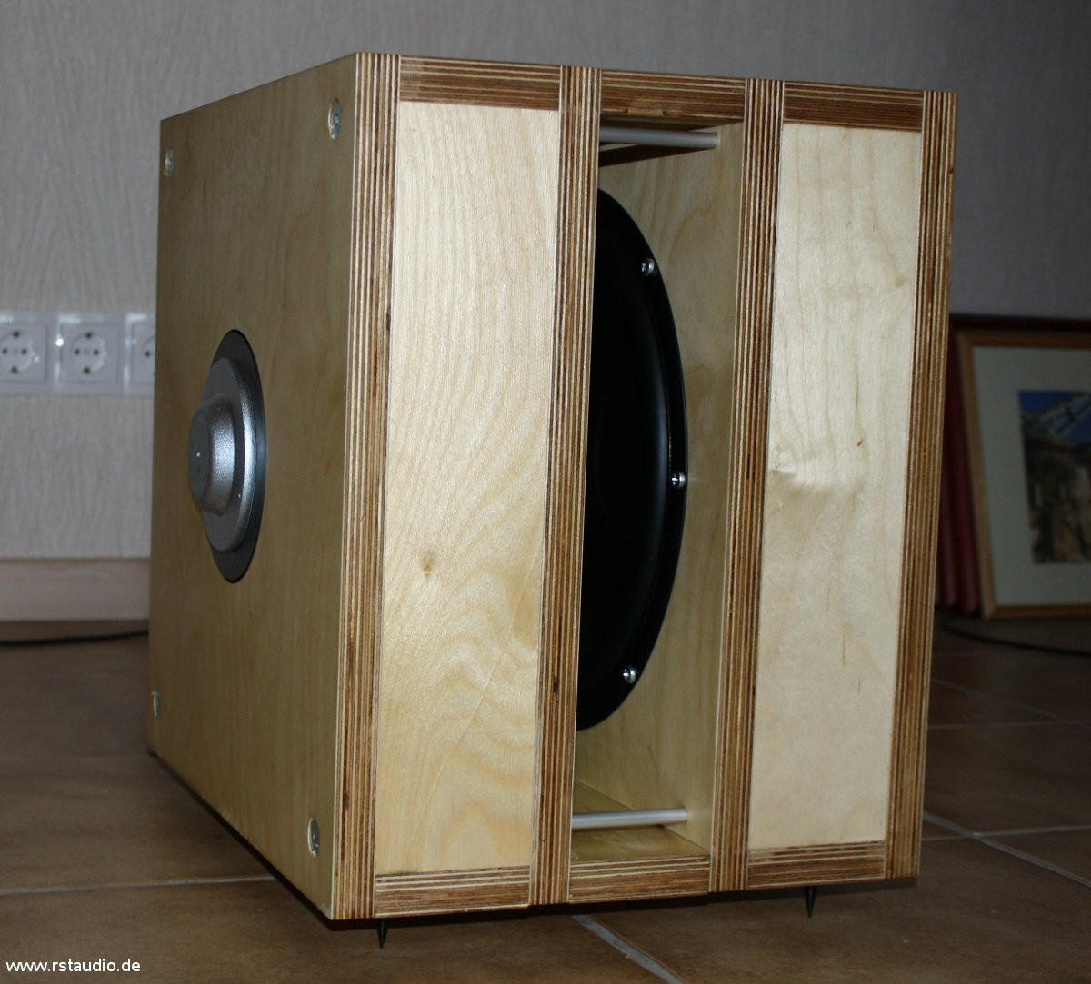
In the meantime, I operate the RiPol without the passive compensation circuit. The two 30cm drivers are thus directly connected to my Hypex power amplifier. A suppression of the resonance frequencies from approx. 250Hz is no longer necessary due to the use of the FIR filters (see below).

I experimented with the crossover frequency between the RiPol and the Quads many years ago and ended up with 125Hz. Since then, I no longer question the result and also use it with the FIR crossover.

Digital Signal Processing

19-03-2022

At this point, one can no longer speak of a simple crossover as with the HQD system. In the early 1980s, the possibilities described here simply did not yet exist.

The stereo signal is digitised and convolved with the help of software (AcourateConvolver) with target functions. The following changes are made to the input signals:

  • 3 way crossover
  • time alignment of the drivers to each other
  • room acoustical correction filters
  • symmetrising the phase between the channels

As a result, you get different output signals for the individual frequency ranges. In the RQM system there are 6 in total, the two Quads of a channel are currently supplied with the same signal and the RiPol receives the bass information of both channels (see below). After D/A conversion, these signals are fed to the corresponding power amplifiers / loudspeakers. With the RQM system, there are a total of 7 hardware channels (1x RiPol, 4x Quads & 2x Mundorfs). I want to keep the option open for the future to treat the Quads individually, so each Quad has its own channel.

One should not underestimate the influence of the measuring equipment! What you don’t capture with a cheap measuring microphone, for example, you can’t correct. This is like comparing a low cost audio system with a high-resolution high-end system. No correction file for the microphone will help, because it only corrects the frequency response and of course does not improve the resolution. In the beginning I used such a microphone (<100€) and today I use an Earthworks M50, the differences were more than clearly audible. Of course, the same applies to the rest of the measuring channel. Naturally, there is also a correction file for an Earthworks microphone.

I use Acourate for all acoustic measurements and calculations. This software is a very powerful, but also extremely complex, tool for digital signal processing. Unfortunately, the documentation leaves much to be desired, even though the Acourate-Wiki is slowly improving. Learning how to use it without outside help seems almost impossible myself. Fortunately, I have my friend and mentor Heiner, who always helps me with advice and support on this complex path.

How to operate Acourate can be read here in detail.

In the following, a detailed description of my measures for the RQM system will emerge over time, which I hope will be helpful for one or the other of you. You can also find more information on the following pages:

Digital Crossover

A digital crossover, as described here, is employed. I still use 2nd order UB jPol11 FIR filters with linear phase. Also the number of TAP’s of 131072 have remained the same. Of course, a 3 way crossover with the crossover frequencies described above (125Hz & 7.5kHz) is needed here.

3 way FIR Crossover

The picture above shows the currently used crossover for the left channel. In the transition frequencies the crossovers have the desired attenuation of -6dB and then drop very steeply.

A crossover is created in Acourate with the help of the menu point “Generate → Crossover”.

Creating my crossover in Acourate

Acourate generates a total of 6 files from these inputs:

  • XO1L96.dbl, XO1R96.dbl
  • XO2L96.dbl, XO2R96.dbl
  • XO3L96.dbl, XO3R96.dbl

“XO” is used to identify a crossover file, “96” provides information about the underlying clock frequency, “L” and “R” of course indicate the left or right channel and the number informs about the frequency range. Acourate starts counting in the bass range. Translated to the RQM system described here, this means:

  1. RiPol – up to 125Hz
  2. Quads – from 125Hz to 7.5kHz
  3. Mundorfs – from 7.5kHz

At this point I wondered at the beginning how to create a crossover for a mono subwoofer? The same way as just described. To operate such a subwoofer, take the final subwoofer files (numbered 1) and feed them both to the output of the mono bass driver, each with a level reduced by -6dB. The signals for the left and right channels are added correctly. An explanation of this can also be found here.

You can also read about the creation of crossovers in the Acourate-Wiki.

Adjustment of the Levels

Before going deeper into Acourate, the levels in the individual signal channels should be adjusted to each other. Acourate naturally corrects these differences, but with larger deviations this is at the expense of the digital “headroom”. In order to lose as little resolution as possible, it is therefore advisable to find a suitable level setting for your own system.

The RQM system with uncorrected Levels

The measurement above shows the amplitude response of the RQM system after smoothing with Macro 1. The maximum level is found at approx. 40Hz with 23dB and the minimum level at approx. 6kHz with -4.5dB. This results in a difference of 27.5 dB.

The RQM system with corrected Levels

I adjust the levels with the VV7, so it does not affect the digital signal processing. I lowered the bass and the treble appropriately. Now the maximum is at 18dB and the minimum at 1dB, a difference of 17dB. Compared to the original setting, I gain more than 10dB.

Time Alignment

Of course, the individual speakers do not have the same distance to the listening position. For this reason, the transit times have to be adjusted. There are several ways to determine these times in Acourate.

The procedure described here shifts the individual files of the crossover in a defined way. The high frequency (XO3x) is taken as reference and left in its original state. The low frequency (XO1x) is shifted by -4000 samples and the midrange (XO2x) by -2000 samples (TD Functions → Rotation). To do this, load the crossover files into curves 1 to 3 (see above). Since the crossover files for the left and right channels are identical, it is sufficient to load only the 3 files of a channel. Then the corresponding curves are shifted and saved as left and right files. Only the currently active curve is moved by the “Signal Rotation” window.

Rotation of XO1x by -4000 Samples

The new files created in this way are transferred to the AcourateConvolver in order to subsequently perform a LogSweep measurement with them. For this purpose, the XO*.dbl files must be converted to XO*.cpv. The following picture shows the impulse response of this measurement (Time). For a better overview, I evaluate the two channels one after the other.

Impulse Response of the left Cannel (Time)

The largest impulse is the treble, the smaller one in front of it is the midrange, and the small waves in front of it are the bass. If we had perfect timing between the individual speakers, the midrange impulse would be exactly 2000 samples before the tweeter impulse and the bass would be 4000 samples before it. The deviations from this are the times we are looking for.

Below the time window, almost exactly in the middle, there is a clock icon. This opens the “Time Alignment Assistant”.

Tweeter Entry in the Left Channel

In “Test Delays for Time Alignment” you enter the shifts that have been made – here they are 0, 2000 and 4000 samples. As you can see, the right channel has already been determined. I will now show you how to do this using the left channel.

Currently we have not zoomed the measurement. The maximum impulse in the measurement window is the high frequency. At a measuring frequency of 96 kHz, this is exactly at 12000 samples – it is programmed into Acourate. A click on “Left Peak” takes over the position of the largest impulse in the activated window. As expected, 12000 appears in the “Left” window. Afterwards, we leave the assistant with “Exit”.

In the Time window we now zoom out the midrange impulse so that the larger impulses of the high frequency are no longer visible.

Time Measurement zoomed by the Midrange Impulse

Now we go back to the Time Alignment Assistant.

Midrange Entry in the Left Channel

Click on “Left Peak” and 10014 appears. If there were no deviation between the high and mid tones, 10000 would be displayed here.

The next step is the bass impulse. Here, too, the area must first be zoomed in accordingly. However, the bass impulse is very small and therefore difficult to recognise. But we know that it has to be about 21ms before the midrange impulse, which corresponds to 2000 samples at a measuring frequency of 96kHz. In addition, I have set the y-axis from “Auto” to ±0.05, so the pulse is easier to identify.

Bass pulse zoomed

In the picture above, the measurement section is not quite correct. At the right edge you can see the beginning of the midrange impulse. Before you take over the values, you have to adjust the zoom again – the “peak” at approx. 0.082s should be the highest in the window. Leave the left marker at its position and set the right marker to e.g. 0.094s. Then zoom in again.

After adjusting the image section, we return to the Time Alignment Assistant.

Bass Entry

Again, clicking on “Left Peak” adds the value to the list. Now all maximum impulses for both channels are determined. The values for the left and right channels are identical for me, which speaks for the set-up and for the exactly central positioning of the measuring microphone.

Thankfully, Acourate takes over the calculation. With a click on “Compute Delays” you finally get:

Calculation of the Delay Times

We see that the bass has to be delayed by 1.66ms and the two tweeters by 0.15ms compared to the midrange. These values are entered into the transfer matrix of the AcourateConvolver.

The values are logical, the mono subwoofer is in the middle and thus closest to my listening position. The tweeters are also somewhat closer to that position. Consequently, these channels have to be delayed. However, I had problems interpreting the values and so I took paper and pencil and recalculated it.


Calculation of the propagation delays from the determined values.

The pulse of the midrange starts at 10014, but should start at 10000. The midrange is therefore delayed. The pulse of the woofer starts at 7855, but should start at 8000. So the woofer comes too early.

First, the shifts in the signals are subtracted from the results – manually (TD Functions → Rotation) and by Acourate (12000):

    \begin{eqnarray*} S_{HT} & = & 12000 - 12000 = 0\\ S_{MT} & = & 10014 - (12000 - 2000) = 14\\ S_{TT} & = & 7855 - (12000 - 4000) = -145 \end{eqnarray*}

Positive values here therefore mean a delayed and negative a premature reaction.

In order to correct the RQM system correctly in terms of time, the low frequency must be delayed by 145 samples and the midrange must be transmitted 14 samples earlier. However, it is not possible to play a signal earlier, because the system would have to be able to look into the future. Digital signals, by contrast, can be delayed very easily.

As a solution to the dilemma, we now additionally delay all speakers by the largest positive value of the samples determined above, in this case 14, and get:

    \begin{eqnarray*} S_{HT} & = & 0 - 14 = -14\\ S_{MT} & = & 14 - 14 = 0\\ S_{TT} & = & -145 - 14 = -159 \end{eqnarray*}

Now all time shifts are ≤0 samples. The signals therefore remain the same (0 samples) or must be delayed (<0 samples). This result can also be seen above in the “Time Alignment Assistant” window.


The biggest problem with this method is the very low bass impulse. In my case, finding the maximum was relatively easy, but there are other speaker setups where this is impossible. For this one uses the method described above with the exception of the bass channel. A suitable method to exactly determine the delay times for more difficult bass systems is described in the article “Time Alignment of Drivers by Sinewave Convolution” by Dr. Ulrich Brüggemann.

Room Acoustic Correction Filters

After the loudspeaker system has been tuned, the room acoustic correction filters can be applied. Of course, the first step is a measurement with Acourate (LogSweep). The AcourateConvolver runs the crossover with the time delays determined above. I measure between 10Hz and 30kHz with a duration of 60s. To generate the correction files, Acourate has so-called macros that do a lot of the work for you, and you can achieve impressive results very quickly.

LogSweep measurement of the RQM system with crossover and delay times

The result is first smoothed with Macro 1.

Acourate Macro 1

The values entered in the “Frequency Dependent Window” come from my friend Heiner. I experimented with them, but always came back to them. This also applies to settings in Macro 4 (see below). If you are creating your correction files for the first time, you should start with the standard settings. After running Macro 1, the result is:

LogSweep measurement after smoothing with Macro 1

To the human eye, the result already looks a little better. With these curves we now move on to the decisive step, the determination of the target curve in Macro 2.

Determining the Target Curve in Macro 2

With my current target curve, the “basic” curve goes classically up to 1kHz and then bends down to -3dB at 20kHz – this corresponds to -3.85dB at 48kHz. That is the starting situation. In addition, I have a “low shelf” with +0.5dB below 150Hz, this small boost has proven itself in many tests. In the upper frequency range I use a “HF Roll Off” of -3dB at 30kHz. The measured curve bends more, but this is due to the fact that I “only” measured up to 30 kHz. The Mundorfs can transmit even higher frequencies.

I listened for about a year with active room correction, but without Mundorf AMT. During this time I preferred a “kink point” at 500Hz. But the shift to 1kHz is much more comfortable for me with the AMT.

The whole task can be created graphically in the Macro 2 window. However, I prefer to directly edit the file “Target.tgt” in the current working directory of Acourate using the text editor.

The decisive factor in the correction is where to place the described curve (y-axis). I have decided on 4dB. This determines which frequency ranges can be corrected (above the target curve) and which cannot (below the target curve). The lower you set the target curve, the more is corrected, but you also lose digital “headroom”.

With “Save Target” the generated target curve is saved. It is shown as the brown curve in the amplitude graph below.

Changing the target curve is an everlasting “playground”. At this point, it is worth trying out many things to get closer to one’s own optimum – e.g. my experiments with the “kink point” or the “low shelf”. Once you have reached this point, you have realised for some time that the noble goal of bringing the concert hall into your listening room is not achievable. In fact, the goal is to sit in front of your own system and be completely satisfied with what you hear.

The next step is Macro 3, where the inverse is formed using the target curve just defined.

Calculation of the Inverse with Macro 3

There is nothing to select for the RQM system in this macro. It is simply executed with a click on “Run Macro3”. The result is displayed in the active window for the amplitudes:

Amplitude Curve of the Measurement, Target Curve and Calculated Inverse

The last step is to execute macro 4.

Calculation of the Correction Files with Macro 4

As already mentioned above, I got the values in “Excessphase window” from my friend Heiner as a recommendation. Of course, you can start with the standard values. But I myself prefer the recommended values, they have been optimised over many years.

Under “Filter sample rate” I always activate all clock frequencies with which my Lynx converter works, although my standard frequency is 96 kHz. Additionally, I create a subsonic filter at 25Hz. Under “Add. output format” I have to select AcourateConvolver CPV and get the required correction files for this programme.

At the top right of the window you can see that the macro has recognised the existence of the files for a 3-way crossover. They are included in the calculation. A click on “Run Macro4” now creates all necessary correction files. The result is the six correction files for 96 kHz in the current working directory of Acourate:

  • Cor1L96.cpv, Cor1R96.cpv
  • Cor2L96.cpv, Cor2R96.cpv
  • Cor3L96.cpv, Cor3R96.cpv

And of course those of the other selected frequencies. I get a total of 36 files. They follow the same naming convention as described above for the crossover files. These files must now be stored for the AcourateConvolver and added to the transfer matrix.

Once you have run the correction files, you have already gone very very far. From here on, there are only small steps that can be taken. In a high-end audio system, however, every small step forward is worthwhile.

Symmetry / ICPA

Once the correction filters have been calculated, the next step is to create symmetry between the two channels. Only corrections to the phase of the signals are made. In Acourate, this calculation is called Inter Channel Phase Alignment (ICPA) and is calculated with Macro 6. A short excerpt of the description by Dr. Ulrich Brüggemann can be found here. In addition, every user of version 2 has the document “ICPA – The Optimisation of Unbalanced Stereo Setups” as a pdf file on the computer with Acourate.

The optimisation is done by alternately using Macro 4 and Macro 6. Macro 4 is first run without the additional frequency calculations and the *.cpv generation. You can see in the picture below that “ICPA” is greyed out the first time it is called up. In the working directory of Acourate there are no files with the phase compensation filters.

First Start of Macro 4

After the first execution of Macro 4, Macro 6 can be called up. For the RQM system I get

First Call of Macro 6 at the RQM system

The peaks below Q=10 (orange line) are compensated in their own channel. For the RQM system, these are the two peaks at approx. 81Hz. All peaks above Q=10 but below Q=60 (the purple line) are reproduced in the other channel. Here it is the peaks at 148Hz and 152Hz. All peaks greater than Q=60 remain uncorrected.

I have got into the practice of compensating for a peak and then running Macro 4 again. After calling Macro 6 again, you can see directly how well the peak was compensated or reproduced. Then I move on to the next peak …

To determine the peak, it is best to first zoom in on the peak to be processed and then place the marker on the peak. Do not forget to select the correct channel under “Source”. With “1. Get Marked Frequency” you take over the values in “f0 [Hz]” and “Q”. These values can then be changed with the arrow buttons. With “2. Demo Edited Values” the changed curve is displayed. If you are satisfied with the result, click on “3. Simulate + Optimize”. Then you can see how the setting affects the phase. If you are satisfied with the correction, it is saved with “4. Save Result”. The setting appears in one of the two upper windows. If the results are marked with “/ macro4”, they have already been calculated with this macro. Macro 6 is exited with a click on “Exit”, but the corrections determined up to that point are not lost.

Macro 6 in the RQM System with the Corrected Peaks

The picture above was taken after determining all 4 peaks relevant for the RQM system. The compensation at 81Hz is perfect, the reproductions at approx. 150Hz quite reasonable. In any case, I am satisfied with the result.

Finally, Macro 4 is called again. This time, however, the additional frequencies and the *.cpv files are generated (see above).

Calling Macro 4 after optimisation with Macro 6

The checkmark in front of “ICPA” is set by Acourate automatically if it finds corresponding results in the current working directory. This way, the ICPA results are included in the correction files. If you do not want this, you can also remove the checkmark in front of “ICPA”.

Audiophile Review

13-04-2022

With all the actions described here, audio transmission in my listening room has once again taken a significant step forward. Since the refurbishment of the Quads in 2020, and especially with the switch to digital signal processing at the beginning of 2021, I have gone from one success to the next. I would never have thought it possible that I would one day be at this point. The new frames and the Mundorf AMT have once again provided significant improvements. I can only strongly recommend anyone using an active multi-way system to look into digital signal processing. I am sure that you will NEVER regret this step.